Aggregate Planning

1. 13 Aggregate Planning

2. Learning Objectives • Explain what aggregate planning is and how it is useful. • Identify the variables decision makers have to work with in aggregate planning and some of the possible strategies they can use. • Describe some of the graphical and quantitative techniques planners use. • Prepare aggregate plans and compute their costs.

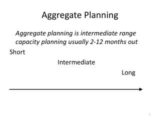
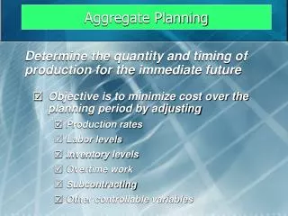
3. Planning Horizon Long range Intermediate range Short range Now 2 months 1 Year Aggregate planning: Intermediate-range capacity planning, usually covering 2 to 12 months.

4. Overview of Planning Levels • Short-range plans (Detailed plans) • Machine loading • Job assignments • Intermediate plans (General levels) • Employment • Output • Long-range plans • Long term capacity • Location / layout

5. Planning Sequence Economic, competitive, and political conditions Corporate strategies and policies Aggregate demand forecasts Establishes operations and capacity strategies Business Plan Establishes operations capacity Aggregate plan Establishes schedules for specific products Master schedule Figure 13.1

6. Aggregate Planning • Begin with forecast of aggregate demand • Forecast intermediate range • General plan to meet demand by setting • Output levels • Employment • Finished goods inventory level • Production plan is the output of aggregate planning • Update plan periodically – rolling planning horizon always covers the next 12 – 18 months

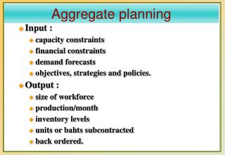
7. Aggregate Planning Inputs Costs Inventory carrying Back orders Hiring/firing Overtime Inventory changes Subcontracting Resources Workforce Facilities Demand forecast Policies Subcontracting Overtime Inventory levels Back orders

8. Aggregate Planning Outputs • Total cost of a plan • Projected levels of inventory • Inventory • Output • Employment • Subcontracting • Backordering

9. Aggregate Planning Strategies • Proactive • Alter demand to match capacity • Reactive • Alter capacity to match demand • Mixed • Some of each

10. Demand Options • Pricing • Promotion • Back orders • New demand

11. Capacity Options • Hire and layoff workers • Overtime/slack time • Part-time workers • Inventories • Subcontracting

12. Aggregate Planning Strategies • Maintain a level workforce • Maintain a steady output rate • Match demand period by period • Use a combination of decision variables

13. Basic Strategies • Level capacity strategy: • Maintaining a steady rate of regular-time output while meeting variations in demand by a combination of options. • Chase demand strategy: • Matching capacity to demand; the planned output for a period is set at the expected demand for that period.

14. Chase Approach • Advantages • Investment in inventory is low • Labor utilization in high • Disadvantages • The cost of adjusting output rates and/or workforce levels

15. Level Approach • Advantages • Stable output rates and workforce • Disadvantages • Greater inventory costs • Increased overtime and idle time • Resource utilizations vary over time

16. Techniques for Aggregate Planning • Determine demand for each period • Determine capacities for each period • Identify policies that are pertinent • Determine units costs • Develop alternative plans and costs • Select the best plan that satisfies objectives. Otherwise return to step 5.

17. Cumulative Graph Cumulative output/demand Cumulative production Cumulative demand 6 7 1 2 3 4 5 8 9 10 Figure 13.3

18. Average Inventory Average inventory Beginning Inventory + Ending Inventory = 2

19. Mathematical Techniques Linear programming: Methods for obtaining optimal solutions to problems involving allocation of scarce resources in terms of cost minimization. Simulation models: Computerized models that can be tested under different scenarios to problems.

20. Summary of Planning Techniques Table 13.7

21. Aggregate Planning in Services • Services occur when they are rendered • Demand for service can be difficult to predict • Capacity availability can be difficult to predict • Labor flexibility can be an advantage in services

22. Aggregate Plan to Master Schedule AggregatePlanning Disaggregation MasterSchedule Figure 13.4

23. Disaggregating the Aggregate Plan • Master schedule: The result of disaggregating an aggregate plan; shows quantity and timing of specific end items for a scheduled horizon. • Rough-cut capacity planning: Approximate balancing of capacity and demand to test the feasibility of a master schedule.

24. Master Scheduling • Master schedule • Determines quantities needed to meet demand • Interfaces with • Marketing • Capacity planning • Production planning • Distribution planning

25. Master Scheduler • Evaluates impact of new orders • Provides delivery dates for orders • Deals with problems • Production delays • Revising master schedule • Insufficient capacity

26. Master Scheduling Process Inputs Outputs Beginning inventory Projected inventory Master Scheduling Forecast Master production schedule Customer orders Uncommitted inventory Figure 13.6

27. Projected On-hand Inventory Projected on-handinventory Inventory fromprevious week Current week’srequirements - =

28. Beginning Inventory Forecast is larger than Customer orders in week 3 Customer orders are larger than forecast in week 1 Forecast is larger than Customer orders in week 2 Projected On-hand Inventory Figure 13.8

29. Time Fences Time Fences – points in timethat separate phases of a master schedule planning horizon.

30. Time Fences in MPS Figure 13.12 Period “frozen”(firm orfixed) “liquid”(open) “slushy”somewhatfirm

31. Solved Problems: Problem 1