DCSP-5: Noise
750 likes | 768 Views
This article provides an introduction to the Fourier Transform and its application in analyzing periodic signals. It also discusses the concept of noise in communication systems and its impact on signal integrity.

DCSP-5: Noise
E N D
Presentation Transcript
DCSP-5: Noise Jianfeng Feng Department of Computer Science Warwick Univ., UK Jianfeng.feng@warwick.ac.uk http://www.dcs.warwick.ac.uk/~feng/dcsp.html
Assignment:2015 • Q1: you should be able to do it after last week seminar • Q2: need a bit reading (my lecture notes) • Q3: standard • Q4: standard
Assignment:2015 • Q5: standard • Q6: standard • Q7: after today’s lecture • Q8: load jazz, plot soundsc load Tunejazz plot load NoiseJazz plot
Recap • Fourier Transform for a periodic signal { sim(n w t), cos(n w t)} • For general function case,
Recap: this is all you have to remember (know)? • Fourier Transform for a periodic signal { sim(n w t), cos(n w t)} • For general function case,
Dirac delta function Can you do FT for cos(2 p t)?
Dirac delta function For example, take F=0 in the equation above, we have It makes no sense !!!!
Dirac delta function: A photo with the highest IQ (15 NL) Shordiger Heisenberg Ehrenfest Bragg Dirac Compton Bone Pauli Debije De Boer M Curie Einstein Planck Lorentz Langevin
Dirac delta function: A photo with the highest IQ (15 NL) Shordiger Heisenberg Ehrenfest Bragg Dirac Compton Bone Pauli Debije De Boer M Curie Einstein Planck Lorentz Langevin
Dirac delta function The (digital) delta function, for a given n0 n0=0 here d(t)
Dirac delta function The (digital) delta function, for a given n0 Dirac delta function d(x) (you could find a nice movie in Wiki); n0=0 here d(t)
Dirac delta function Dirac delta function d(x); The FT of cos(2pt) is -1 0 1 Frequency
A final note (in exam or future) • Fourier Transform for a periodic signal { sim(n w t), cos(n w t)} • For general function case (it is true, but need a bit further work),
Summary Will come back to it soon (numerical) This trick (FT) has changed our life and will continue to do so
This Week’s Summary • Noise • Information Theory
Noise Noise in communication systems: probability and random signals I = imread('peppers.png'); imshow(I); noise = 1*randn(size(I)); Noisy = imadd(I,im2uint8(noise)); imshow(Noisy);
Noise Noise in communication systems: probability and random signals I = imread('peppers.png'); imshow(I); noise = 1*randn(size(I)); Noisy = imadd(I,im2uint8(noise)); imshow(Noisy);
Noise Noise is a random signal (in general). By this we mean that we cannot predict its value. We can only make statements about the probability of it taking a particular value
pdf The probability density function (pdf) p(x) of a random variable x is the probability that x takes a value between x0 and x0 +dx. We write this as follows: p(x0 )dx =P(x0 <x< x0 +dx) P(x) [x0 x0+ dx]
pdf Probability that x will take a value lying between x1 and x2 is The probability is unity. Thus
IQ distribution Above Average 34.1% Exceptionally Gifted 0.13% Low Intelligence 13.6% High Intelligence 13.6% Superior Intelligence 2.1% Mentally Inadequate 23% Average 34.1%
pdf A density satifying the equation is termed normalized. The cumulative distribution function (CDF) F(x) is the probability x is less than x0 My IQ is above 85% (F(my IQ)=85%).
pdf From the rules of integration: P(x1<x<x2) = P(x2) --P(x1) pdf has two classes: continuous and discrete
Continuous distribution An example of a continuous distribution is the Normal, or Gaussian distribution: where m, s is the mean and standard variation value of p(x). The constant term ensures that the distribution is normalized.
Continuous distribution. This expression is important as many actually occurring noise source can be described by it, i.e. white noise or coloured noise.
Generating f(x) from matlab X=randn(1,1000); Plot(x); • X[1], x[2], …. X[1000], • Each x[i] is independent • Histogram
Discrete distribution. If a random variable can only take discrete value, its pdf takes the forms of lines. An example of a discrete distribution is the Poisson distribution
Mean and variance We cannot predicate value a random variable We can introduce measures that summarise what we expect to happen on average. The two most important measures are the mean (or expectation) and the standard deviation. The mean of a random variable x is defined to be
Mean and variance • In the examples above we have assumed that the mean of the Gaussian distribution to be 0, the mean of the Poisson distribution is found to be l.
Mean and variance • The mean of a distribution is, in common sense, the average value. • Can be estimated from data • Assume that {x1, x2, x3, …,xN} are sampled from a distribution • Law of Large Numbers: EX ~ (x1+x2+…+xN)/N
Mean and variance mean • The more data we have, the more accurate we can estimate the mean • (x1+x2+…+xN)/N against N for randn(1,N)
Mean and variance • The variance is defined as The variance s is defined to be • The square root of the variance is called standard deviation. • Again, it can be estimated from data
Mean and variance • The standard deviation is a measure of the spread of the probability distribution around the mean. • A small standard deviation means the distribution are close to the mean. • A large value indicates a wide range of possible outcomes. • The Gaussian distribution contains the standard deviation within its definition (m,s)
Mean and variance • Communication signals can be modelled as a zero-mean, Gaussian random variable. • This means that its amplitude at a particular time has a PDF given by Eq. above. • The statement that noise is zero mean says that, on average, the noise signal takes the values zero.
Mean and variance http://en.wikipedia.org/wiki/Nations_and_intelligence
Einstein’s IQ Einstein’s IQ=160+ What about yours? Above Average 34.1% Exceptionally Gifted 0.13% Low Intelligence 13.6% High Intelligence 13.6% Superior Intelligence 2.1% Mentally Inadequate 23% Average 34.1%
SNR • Signal to noise ratio is an important quantity in determining the performance of a communication channel. • The noise power referred to in the definition is the mean noise power. • It can therefore be rewritten as SNR= 10 log10 ( S / s2)
Correlation or covariance • Cov(X,Y) = E(X-EX)(Y-EY) • correlation coefficient is normalized covariance Coef(X,Y) = E(X-EX)(Y-EY) / [s(X)s(Y)] • Positive correlation, Negative correlation • No correlation (independent)
Stochastic process = signal • A stochastic process is a collection of random variables x[n], for each fixed [n], it is a random variable • Signal is a typical stochastic process • To understand how x[n] evolves with n, we will look at auto-correlation function (ACF) • ACF is the correlation between k steps
Stochastic process >> clear all close all n=200; for i=1:10 x(i)=randn(1,1); y(i)=x(i); end for i=1:n-10 y(i+10)=randn(1,1); x(i+10)=.8*x(i)+y(i+10); end plot(xcorr(x)/max(xcorr(x))); hold on plot(xcorr(y)/max(xcorr(y)),'r') • two signals are generated: y (red) is simply randn(1,200) x (blue) is generated x[i+10]=.8*x[i] + y[i+10] • For y, we have g(0)=1, g(n)=0, if n is not 0 : having no memory • For x, we have g (0)=1, and g (n) is not zero, for some n: having memory
white noise w[n] • White noise is a random process we can not predict at all (independent of history) • In other words, it is the most ‘violent’ noise • White noise draws its name from white light which will become clear in the next few lectures
white noise w[n] • The most ‘noisy’ noise is a white noise since its autocorrelation is zero, i.e. corr(w[n], w[m])=0 when • Otherwise, we called it colour noise since we can predict some outcome of w[n], given w[m], m<n
Sweety Gaussian Why do we love Gaussian?
Sweety Gaussian Yes, I am junior Gaussian + = Herr Gauss + Frau Gauss = Juenge Gauss • A linear combination of two Gaussian random variables is Gaussian again • For example, given two independent Gaussian variable X and Y with mean zero • aX+bY is a Gaussian variable with mean zero and variance a2 s(X)+b2s(Y) • This is very rare (the only one in continuous distribution) but extremely useful: panda in the family of all distributions
DCSP-6: Information Theory Jianfeng Feng Department of Computer Science Warwick Univ., UK Jianfeng.feng@warwick.ac.uk http://www.dcs.warwick.ac.uk/~feng/dcsp.html
Data Transmission How to deal with noise? How to transmit signals?
Data Transmission Transform I • Fourier Transform • ASK (AM), FSK(FM), and PSK (skipped, but common knowledge) • Noise • Signal Transmission