Linear Classification Models: Generative

1. Linear Classification Models:Generative Prof. NavneetGoyal CS & IS BITS, Pilani

2. Perceptron

3. Approaches to Classification • Probabilistic • Inference stage – use training data to learn a model for p(Ck|x) • Decision stage – use posterior probabilities p(Ck|x) to make optimal class assignments • Discriminant fn. • Solve both problems together and simply learn a fn. that maps x directly to a class • Probabilistic • Generative • First solve inference problem of determining class conditional densities p(x|Ck) for each class Ck and then determine posterior probabilities • Discriminative

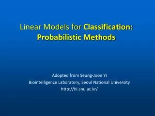
4. Probabilistic Models • Probabilistic view of classification! • Models with linear decision boundaries arise from simple assumptions about the distribution of data • Two approaches: • Generative Models (2 steps) • Discriminative Models (1 step) • In both cases use decision theory to assign a new x to a class

5. Probabilistic Generative Models • 2 step process • Model class conditional densities p(x|Ck) & class priors p(Ck) • Use them to compute class posterior probabilities p(Ck|x) according to Bayes’ theorem • 2 class case • Posterior prob. for class C1 = p(C1|x) = σ (a), the logistic sigmoid fn. • a = & • Sigmoid fn is S-shaped and is also called the squashing fn because it maps the whole real line into a finite interval (maps real a ε (-∞, +∞) to finite (0,1) interval) • Plays an important role in many classification algorithms

6. Probabilistic Generative Models • Symmetry property • Inverse of the logistic sigmoid fn is given by & is called the logit or log odds function because it represents the log of the ratio of the probabilities for the 2 classes

7. Probabilistic Generative Models • Posterior probabilities have been written in an equivalent form using σ! p(C1|x) = σ (a) • What’s the significance of doing so? • We shall see this shortly when a(x) takes a simple functional form • If a(x) is a linear fn. of x, then then posterior prob. is governed by a generalized linear model • Generalized Linear Model?

8. Probabilistic Generative Models Generalized Linear Model • In linear regression models, the model prediction y(x,w)was given by a linear function of the parameters w • In the simplest case, the model is also linear in the input variables x so that y is a real no. • In classification, we wish to predict discrete class labels, or more generally posterior probabilities in (0,1) • To achieve this, we consider a generalization of this model in which we transform the linear fn of w using a non-linear fn f(.) so that In ML, f(.) is know as an activation fn., whereas its inverse is called a link fn. in statistical literature

9. Probabilistic Generative Models Generalized Linear Model • Decision surface corresponds to so that • Decision surfaces are linear fns of x, even if the fn f(.) is non-linear • Generalized linear models are no longer linear in the parameters due to non-linear fn f(.) • More complex in terms of analytical and computational properties! • Still simpler that the more general non-linear models

10. Probabilistic Generative Models K>2 classes: Softmax Function

11. Probabilistic Generative Models K>2 classes: Softmax Function

12. Probabilistic Generative Models Softmax Function

13. Probabilistic Generative Models Softmax Function

14. Probabilistic Generative Models Softmax Function The soft maximum approximates the hard maximum and is a convex function just like the hard maximum. But the soft maximum is smooth. It has no sudden changes in direction and can be differentiated as many times as you like. These properties make it easy for convex optimization algorithms to work with the soft maximum. In fact, the function may have been invented for optimization;

15. Probabilistic Generative Models Softmax Function • Accuracy of the soft maximum approximation depends on scale • Multiplying x and y by a large constant brings the soft maximum closer to the hard maximum • For example, g(1, 2) = 2.31, but g(10, 20) = 20.00004 • “hardness” of the soft maximum can be controlled by generalizing the soft maximum to depend on a parameter k. • g(x, y; k) = log( exp(kx) + exp(ky) ) / k • Soft maximum can be made as close to the hard maximum as desired by making k large enough • For every value of k the soft maximum is differentiable, but the size of the derivatives increase as k increases. • In the limit the derivative becomes infinite as the soft maximum converges to the hard maximum

16. Probabilistic Generative Models • Forms of class-conditional densities • Continuous Inputs (x follows Gaussian distribution) • Discrete Inputs (for example )

17. Posterior Porbability p(C1|X) Class conditional densities

18. Probabilistic Generative Models • Continuous Inputs (x follows Gaussian distribution) • All classes share the same covariance matrix • All classes do not share the same covariance matrix

19. Probabilistic Discriminative Models • Logistic Regression • 2-class • Multi-class • Parameters using • Maximum Likelihood • Iterative Reweighted Least Squares (IRLS) • Probit Regression

20. Probabilistic Discriminative Models • Logistic Regression • Logistic regression is a form of regression analysis in which the outcome variable is binary or dichotomous • Consider a binary response variable • Variable with two outcomes • One outcome represented by a 1 and the other represented by a 0 • Examples: Does the person have a disease? Yes or No Who is the person voting for? McCain or Obama Outcome of a baseball game? Win or loss

21. Probabilistic Discriminative Models • Logistic Regression Example Data Set • Response Variable –> Admission to Grad School (Admit) • 0 if admitted, 1 if not admitted • Predictor Variables • GRE Score (gre) • Continuous • University Prestige (topnotch) • 1 if prestigious, 0 otherwise • Grade Point Average (gpa) • Continuous

22. Probabilistic Discriminative Models • First 10 Observations of the Data Set ADMIT GRE TOPNOTCH GPA 1 380 0 3.61 0 660 1 3.67 0 800 1 4 0 640 0 3.19 1 520 0 2.93 0 760 0 3 0 560 0 2.98 1 400 0 3.08 0 540 0 3.39 1 700 1 3.92

23. Consider the linear probability model Issue: π(Xi) can take on values less than 0 or greater than 1 Issue: Predicted probability for some subjects fall outside of the [0,1] range. Logistic Regression

24. Consider the logistic regression model GLM with binomial random component and identity link g(μ) = logit(μ) Range of values for π(Xi) is 0 to 1 Logistic Regression

25. Consider the logistic regression model And the linear probability model Then the graph of the predicted probabilities for different grade point averages: Logistic Regression

26. What is Logistic Regression? • In a nutshell: A statistical method used to model dichotomous or binary outcomes (but not limited to) using predictor variables. Used when the research method is focused on whether or not an event occurred, rather than when it occurred (time course information is not used).

27. What is Logistic Regression? • What is the “Logistic” component? Instead of modeling the outcome, Y, directly, the method models the log odds(Y) using the logistic function.

28. Logistic Regression • Simple logistic regression = logistic regression with 1 predictor variable • Multiple logistic regression = logistic regression with multiple predictor variables • Multiple logistic regression = Multivariable logistic regression = Multivariate logistic regression

29. Logistic Regression predictor variables dichotomous outcome is the log(odds) of the outcome.

30. Logistic Regression intercept model coefficients is the log(odds) of the outcome.

31. Odds & Probability

32. Maximum Likelihood • Flipped a fair coin 10 times: T, H, H, T, T, H, H, T, H, H • What is the Pr(Heads) given the data? 1/100? 1/5? 1/2? 6/10?

33. Maximum Likelihood T, H, H, T, T, H, H, T, H, H • What is the Pr(Heads) given the data? • Most reasonable data-based estimate would be 6/10. • In fact, is the ML estimator of p.

34. Maximum Likelihood: Example • Discrete distribution, finite parameter space • How biased an unfair coin is? • Call the probability of tossing a HEAD p. Determine p. • Toss the coin 80 times • Outcome is 49 HEADS and 31 TAILS, • Suppose the coin was taken from a box containing three coins: • one which gives HEADS with probability p = 1/3, • one which gives HEADS with probability p = 1/2 and • another which gives HEADS with probability p = 2/3. • NO labels on these coins • Using maximum likelihood estimation the coin that has the largest likelihood can be found, given the data that were observed. By using the probability mass function of the binomial distribution with sample size equal to 80, number successes equal to 49 but different values of p (the "probability of success"), the likelihood function (defined below) takes one of three values:

35. Maximum Likelihood: Example • Discrete distribution, finite parameter space • The likelihood is maximized when p = 2/3, and so this the maximum likelihood estimate for p.

36. Maximum Likelihood: Example • Discrete distribution, continuous parameter space Now suppose that there was only one coin but its p could have been any value 0 ≤ p ≤ 1. The likelihood function to be maximized is: and the maximization is over all possible values 0 ≤ p ≤ 1. differentiating with respect to p (solutions p = 0, p = 1, and p = 49/80) The solution which maximizes the likelihood is clearly p = 49/80 Thus the maximum likelihood estimator for p is 49/80.

37. Maximum Likelihood: Example Continuous distribution, continuous parameter space • Do it for Gaussian Distribution yourself! • Two parameters, μ & σ Its expectation value is equal to the parameter μ of the given distribution, • which means that the maximum-likelihood estimator μis unbiased. • This means that the estimator is biased. However, is consistent. • In this case it could be solved individually for each parameter. In general, it may not be the case.

38. Maximum Likelihood • The method of maximum likelihood estimation chooses values for parameter estimates (regression coefficients) which make the observed data “maximally likely.” • Standard errors are obtained as a by-product of the maximization process

39. The Logistic Regression Model intercept model coefficients is the log(odds) of the outcome.

40. Maximum Likelihood • We want to choose β’s that maximizes the probability of observing the data we have: Assumption: independent y’s

41. Linear probability model • Obvious possibility is to use traditional linear regression model • But this has problems • Distribution of dependent variable hardly normal • Predicted probabilities cannot be less than 0, greater than 1

42. Linear probability model predictions

43. Logistic regression model • Instead, use logistic transformation (logit) of probability, log of the odds

44. Logistic regression model predictions

45. Estimation of logistic regression model • Least-squares no longer best way of estimating parameters of logistic regression model • Instead use maximum likelihood estimation • Finds values of parameters that have greatest probability, given data

46. Space shuttle data • Data on 24 space shuttle launches prior to Challenger • Dependent variable, whether shuttle flight experienced thermal distress incident • Independent variables • Date – whether shuttle changes or age has effect • Temperature – whether joint temperature on booster has effect

47. First model—date as single independent variable • Dependent variable • Any thermal distress on launch • Independent variable • Date (days since 1/1/60) • SPSS procedure • Regression, Binary logistic

48. Predicted probability of thermal distress using date

49. Exponential of B as change in odds

50. What does “odds” mean? • Odds is the ratio of probability of success to probability of failure • Like odds on horse races • Even odds, odds = 1, implies probability equals 0.5 • Odds = 2 means 2 to 1 in favor of success, implies probability of 0.667 • Odds = 0.5 means 1 to 2 in favor (or 2 to 1 against) success, implies probability of 0.333