Simple Linear Regression

1. Simple Linear Regression

2. Relationship Between Two Quantitative Variables • If we can model the relationship between two quantitative variables, we can use one variable, X, to predict another variable, Y. • Use height to predict weight. • Use percentage of hardwood in pulp to predict the tensile strength of paper. • Use square feet of warehouse space to predict monthly rental cost. L. Wang, Department of Statistics University of South Carolina; Slide 2

3. Simple Linear Regression • Simple: only one predictor variable • Linear: Straight line relationship • Regression: Fit data to (straight line) model y (Response or Dependent Variable) x (Predictor, Regressor, or Independent Variable) L. Wang, Department of Statistics University of South Carolina; Slide 3

4. Use Scatter Plot to See Relationship L. Wang, Department of Statistics University of South Carolina; Slide 4

5. Absorbed Liquid Data • In a chemical process, batches of liquid are passed through a bed containing an ingredient that is absorbed by the liquid. • We will attempt to relate the absorbed percentage of the ingredient (y) to the amount of liquid in the batch (x). L. Wang, Department of Statistics University of South Carolina; Slide 5

6. Absorbed Liquid Data L. Wang, Department of Statistics University of South Carolina; Slide 6

7. Absorbed Liquid Data L. Wang, Department of Statistics University of South Carolina; Slide 7

8. Abs% = -1822 + 435(Amt) The regression line or model is deterministic. L. Wang, Department of Statistics University of South Carolina; Slide 8

9. We are going to use a probabilistic model which accounts for the variation around the line. L. Wang, Department of Statistics University of South Carolina; Slide 9

10. Probabilistic Model • Probabilistic Model: deterministic plus error component for unexplained variation. L. Wang, Department of Statistics University of South Carolina; Slide 10

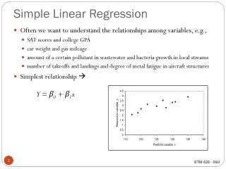
11. Regression Equation y = deterministic model + random error β0 = y-intercept β1 = slope ε = random error Regression line is estimate of the mean value of y at a given value of x. L. Wang, Department of Statistics University of South Carolina; Slide 11

12. Interpreting parameters • Once we determine that a straight line model is reasonable, we want to establish the best line by estimating β0 and β1. µ = E(y) = β0 + β1x • β1is the slope. It is the amount by which y will change with a unit increase in x. • β0 is the y-intercept. It is the expected (mean) value of y when x = 0. (This may or may not be meaningful.) L. Wang, Department of Statistics University of South Carolina; Slide 12

13. If Amount goes up by 1 unit, then the Absorb% is expected to go up by 435 %. If Amount = 0, the expected Absorb% = -1822 units. L. Wang, Department of Statistics University of South Carolina; Slide 13

14. Absorbed Liquid Data Do not consider x values outside the range of the data. L. Wang, Department of Statistics University of South Carolina; Slide 14

15. Errors of Prediction = Vertical Distance Between Points and Line L. Wang, Department of Statistics University of South Carolina; Slide 15

16. Method of Least Squares • Sum of prediction errors = 0. • Sum of the squared errors = Sum of Squares Error = SSE • Many lines for which the sum of errors = 0. • Only one line for which SSE is minimized. • Least squares line = regression line = line for which SSE is minimized. or L. Wang, Department of Statistics University of South Carolina; Slide 16

17. Least Squares Estimates • Deviation of ith point from estimated value: • The sum of the square of deviations for all n points: • Values of and that minimize SSE are called the least squares estimates. They are also the minimum variance unbiased estimates. L. Wang, Department of Statistics University of South Carolina; Slide 17

18. Formulas for Least Squares Estimates where L. Wang, Department of Statistics University of South Carolina; Slide 18

19. Assumptions of a Regression Analysis • Assumptions involve distribution of errors. • Actual errors: • Estimated errors - residuals • Use plots of residuals to check the assumptions. L. Wang, Department of Statistics University of South Carolina; Slide 19

20. There are Four Assumptions (1) The mean of the errors is 0 at each value of x. X values X values YES NO L. Wang, Department of Statistics University of South Carolina; Slide 20

21. Plot of Residuals vs X Values L. Wang, Department of Statistics University of South Carolina; Slide 21

22. There are Four Assumptions (2) Variance of errors is constant across all values of x. X values X values YES NO L. Wang, Department of Statistics University of South Carolina; Slide 22

23. StatCrunch Plot of Residuals vs X Values L. Wang, Department of Statistics University of South Carolina; Slide 23

24. There are Four Assumptions (3) Errors have normal distribution at each x. NO YES L. Wang, Department of Statistics University of South Carolina; Slide 24

25. QQ Plot of Residuals L. Wang, Department of Statistics University of South Carolina; Slide 25

26. There are Four Assumptions (4) Errors are independent – must know how data was gathered. NO YES L. Wang, Department of Statistics University of South Carolina; Slide 26

27. Estimate of Variance at each x, σ2 s is estimated standard error of regression model. L. Wang, Department of Statistics University of South Carolina; Slide 27

28. MSE and Root MSE L. Wang, Department of Statistics University of South Carolina; Slide 28

29. If the variation predicted by the model is significantly larger than the error variation, we have a significant model. L. Wang, Department of Statistics University of South Carolina; Slide 29

30. Coefficient of Determination • Coefficient of Determination, R2, measures the contribution of x in the predicting of y. • Proportion of total sample variation explained by linear relationship: L. Wang, Department of Statistics University of South Carolina; Slide 30

31. Coefficient of Determination • Recall: • SSyy is total sample variation around y. • SSE is unexplained sample variability after fitting regression line. L. Wang, Department of Statistics University of South Carolina; Slide 31

32. Coefficient of Determination = proportion of total sample variability around y that is explained by the linear relationship between y and x. R2 varies from 0 to 1 with large values indicating a good model fit. L. Wang, Department of Statistics University of South Carolina; Slide 32

33. ANOVA Table for Simple Linear Regression L. Wang, Department of Statistics University of South Carolina; Slide 33

34. Amt and Absorb% H0: Model is not significant Ha: Model is significant L. Wang, Department of Statistics University of South Carolina; Slide 34

35. Sampling Distribution of β1 Standard Error for : L. Wang, Department of Statistics University of South Carolina; Slide 35

36. Test of Model Utility H0: β1 = 0 Ha: β1 = 0 Test Statistic: Confidence Interval: L. Wang, Department of Statistics University of South Carolina; Slide 36

37. Amt and Absorb% H0: β1 = 0 Ha: β1 = 0 L. Wang, Department of Statistics University of South Carolina; Slide 37

38. Coefficient of Correlation • Correlation measures the linear relationship between two quantitative variables. • To get a visual picture, use a scatter plot. • To assign a numeric value: Pearson’s coefficient of correlation, r. r is scalar and will vary from –1 to +1. L. Wang, Department of Statistics University of South Carolina; Slide 38

39. Coefficient of Correlation r = -1 r = +1 L. Wang, Department of Statistics University of South Carolina; Slide 39

40. Coefficient of Correlation r = -.80 r = .95 L. Wang, Department of Statistics University of South Carolina; Slide 40 r = 0 r = 0