Download
1 / 30
300 likes | 442 Views
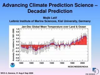
Decadal Climate Prediction. Jochem Marotzke Max Planck Institute for Meteorology (MPI-M) Centre for Marine and Atmospheric Sciences Hamburg, Germany. Outline. A curious apparent paradox… Seamless prediction of weather and climate Examples of decadal climate prediction

E N D
Decadal Climate Prediction Jochem Marotzke Max Planck Institute for Meteorology (MPI-M) Centre for Marine and Atmospheric Sciences Hamburg, Germany
Outline • A curious apparent paradox… • Seamless prediction of weather and climate • Examples of decadal climate prediction • Ocean observations and decadal prediction
A curious apparent paradox… • We confidently predict weather one week into the future… • We confidently state that by 2100, anthropogenic global warming will be easily recognisable against natural climate variability…(cf., IPCC simulations) • Yet we make no statements about the climate of the year 2015
Two types of predictions • Edward N. Lorenz (1917–2008) • Predictions of the 1st kind • Initial-value problem • Weather forecasting • Lorenz: Weather forecasting fundamentally limited to about 2 weeks • Predictions of the 2nd kind • Boundary-value problem • IPCC climate projections (century-timescale) • No statements about individual weather events • Initial values considered unimportant; not defined from observed climate state
Can we merge the two types of prediction? • John von Neumann wrote in 1955: “The approach is to try first short-range forecasts, then long-range forecasts of those properties of the circulation that can perpetuate themselves over arbitrarily long periods of time....and only finally to attempt forecasts for medium-long time periods.”
Seamless prediction of weather and climate • “It is now possible for WCRP to address the seamless prediction of the climate system from weekly weather to seasonal, interannual, decadal and centennial climate variations and anthropogenic climate change.” (WCRP 2005)
Seamless prediction of weather and climate • Combination of predictions of first and second kind – start from observed climate state; include change in concentrations of greenhouse gases and aerosols • Already practiced in seasonal climate prediction (El Niño forecasts) • In decadal prediction, anthropogenic climate change and natural variability expected to be equally important • Atmosphere loses its “memory” after two weeks – any predictability beyond two weeks residing in initial values must arise from slow components of climate system – ocean, cryosphere, soil moisture…
Seamless prediction of weather and climate • Data assimilation & initialisation techniques (developed in weather & seasonal climate prediction) must be applied to ocean, cryosphere, soil moisture • Also “imported” from seasonal climate prediction: building of confidence (“validation”) of prediction system, by hindcast experiments (retroactive predictions using only the information that would have been available at the time the prediction would have been made)
Policy relevance of decadal climate prediction • “Long-term” planning in industry, business & public sector overwhelmingly occurs on the decadal timescale • Adaptation planning to climate change overwhelmingly occurs on the decadal timescale • Clear that, in addition to the multi-decadal mitigation planning & very-long term perspective, decadal timescale is crucial
Examples of decadal climate prediction • Differences arise from models used, but mainly (?) from the method by which the ocean component of coupled model is initialised: • “Optimal interpolation” (Hadley Centre, European Centre for Medium-Range Weather Forecasts) • Forcing of sea surface temperature (SST) in coupled model toward observations (IFM-GEOMAR & MPI-M) • Using 4-dimensional ocean synthesis (ECCO) to initialise ocean component (MPI-M & UniHH)
Hadley Cntr. prediction, global-mean surface temp. D. M. Smith et al., Science 10 August 2007
IFM-GEOMAR & MPI-M decadal prediction Keenlyside et al. (Nature 2008)
Decadal-mean global-mean surface temp. Keenlyside et al. (Nature 2008)
MPI-M & UniHH prediction: N-Atl. SST Annual Assimilation HadISST Hind- & Forecasts Free model Pentadal Decadal Pohlmann et al. (2008)
MPI-M & UniHH prediction: Global SST Annual Assimilation HadISST Hind- & Forecasts Free model Pentadal Decadal Pohlmann et al. (2008)
MPI-M & UniHH prediction: N-Atl. SST HadISST Forecasts Free model Pohlmann et al. (2008)
Organisation of decadal prediction (WCRP) • Decadal prediction is a vibrant effort if one considers the focus on • Ocean initialisation • Atlantic We need to develop broader scope concerning • Areas other than the Atlantic • Roles in initialization of: • Cryosphere • Soil moisture • Stratosphere • The science of coupled data assimilation & initialisation has not been developed yet
Ocean observations and decadal prediction • Initialisation of ocean component of coupled models is the most advanced initialisation aspect of decadal prediction • Yet, methodological uncertainties are huge • Example: Meridional Overturning Circulation (MOC) in the Atlantic • Take-home message: Comprehensive and long-term in-situ and remotely-sensed observations are crucial
North Atlantic Meridional Overturning Circulation (a.k.a. Thermohaline Circulation) Quadfasel (2005)
Bryden et al. (2005) ECMWF MOC at 25N in ocean syntheses (GSOP)
Monitoring the Atlantic MOC at 26.5°N(Marotzke, Cunningham, Bryden, Kanzow, Hirschi, Johns, Baringer, Meinen, Beal) Data recovery: April, May, Oct. 2005; March, Mai, Oct., Dec. 2006, March, Oct2007, March 2008 Church (SCIENCE, 17. August 2007)
Monitoring the Atlantic MOC at 26.5°N(Marotzke, Cunningham, Bryden, Kanzow, Hirschi, Johns, Baringer, Meinen, Beal)
Monitoring the Atlantic MOC at 26.5°N(Marotzke, Cunningham, Bryden, Kanzow, Hirschi, Johns, Baringer, Meinen, Beal)
First observed MOC time series, 26.5N Atlantic Florida Current MOC Ekman Geostro-phic upper mid-ocean S. A. Cunningham et al., Science (17 August 2007)
Modelled vs. observed MOC variability at 26.5N Correlation Observations ECCO (Ocean Synthesis) ECHAM5/MPI-OM RMS variability Baehr et al. (2008)
Update – 2.5 years of MOC time series at 26.5 N Kanzowet al. (2008, in preparation)
Outlook – MOC monitoring at 26.5N • Dec. 2007: NERC will continue the funding for MOC monitoring until 2014 • Transformation into operational array must take place during that period • Data need to enter data assimilation system, to be used in initialising global coupled climate models • Symbiosis of sustained observations and climate prediction (analogy to atmospheric observations and weather prediction)
Conclusions and outlook (1) • Climate prediction up to a decade in advance is possible, as shown by predictive skill of early, relatively crude efforts • Desirable: multi-year seasonal averages, several years in advance, on regional scale • Sustained (operational-style) observations crucial
Conclusions and outlook (2) Large potential for methodological improvement: • Initialisation beyond ocean-atmosphere (cryosphere, soil moisture) • Development of coupled data assimilation (challenge: disparate timescales) • Provision of uncertainty estimate by ensemble prediction – challenge: • Construct ensemble spanning range of uncertainty in initial values; • Poorly known which processes dominate error growth on decadal timescale) • Increase in model resolution for regional aspects • Vast increase in computer power required