Graphical Models in Machine Learning
Graphical Models in Machine Learning. AI4190. Outlines of Tutorial. 1. Machine Learning and Bioinformatics Machine Learning Problems in Bioinformatics Machine Learning Methods Applications of ML Methods for Bio Data Mining 2. Graphical Models Bayesian Network


Graphical Models in Machine Learning
E N D
Presentation Transcript
Outlines of Tutorial 1. Machine Learning and Bioinformatics • Machine Learning • Problems in Bioinformatics • Machine Learning Methods • Applications of ML Methods for Bio Data Mining 2. Graphical Models • Bayesian Network • Generative Topographic Mapping • Probabilistic clustering • NMF (nonnegative matrix factorization)
Outlines of Tutorial 3. Other Machine Learning Methods • Neural Networks • K Nearest Neighborhood • Radial Basis Function 4. DNA Microarrays 5. Applications of GTM for Bio Data Mining • DNA Chip Gene Expression Data Analysis • Clustering the Genes 6. Summary and Discussion * References
knowledge knowledge Machine learning Bio DB medical therapy research Drug Development Pharmacology Ecology 1. Machine Learning and Bioinformatics
Machine Learning • Supervised Learning • Estimate an unknown mapping from known input- output pairs • Learn fw from training set D={(x,y)} s.t. • Classification: y is discrete, categorical • Regression: y is continuous • Unsupervised Learning • Only input values are provided • Learn fw from D={(x)} • Compression • Clustering
Machine Learning Methods • Probabilistic Models • Hidden Markov Models • Bayesian Networks • Generative Topographic Mapping (GTM) • Neural Networks • Multilayer Perceptrons (MLPs) • Self-Organizing Maps (SOM) • Genetic Algorithms • Other Machine Learning Algorithms • Support Vector Machines • Nearest Neighbor Algorithms • Decision Trees
Applications of ML Methods for Bio Data Mining (1) • Structure and Function Prediction • Hidden Markov Models • Multilayer Perceptrons • Decision Trees • Molecular Clustering and Classification • Support Vector Machines • Nearest Neighbor Algorithms • Expression (DNA Chip Data) Analysis: • Self-Organizing Maps • Bayesian Networks • Generative Topographic Mapping • Bayesian Networks • Gene Modeling Gene Expression Analysis • [Friedman et al., 2000]
Applications of ML Methods for Bio Data Mining (2) • Multi-layer Perceptrons • Gene Finding / Structure Prediction • Protein Modeling / Structure and Function Prediction • Self-Organizing Maps (Kohonen Neural Network) • Molecular Clustering • DNA Chip Gene Expression Data Analysis • Support Vector Machines • Classification of Microarray Gene Expression and Gene Functional Class • Nearest Neighbor Algorithms • 3D Protein Classification • Decision Trees • Gene Finding: MORGAN system • Molecular Clustering
2. Probabilistic Graphical Models • Represent the joint probability distribution on some random variables in compact form. • Undirected probabilistic graphical models • Markov random fields • Boltzmann machines • Directed probabilistic graphical models • Helmholtz machines • Bayesian networks • Probability distribution for some variables given values of other variables can be obtained in a probabilistic graphical model. • Probabilistic inference.
Classes of Graphical Models Graphical Models Undirected Directed - Boltzmann Machines - Markov Random Fields - Bayesian Networks • Latent Variable Models - Hidden Markov Models - Generative Topographic Mapping • Non-negative Matrix Factorization
Bayesian Networks A graphical model for probabilistic relationships among a set of variables • Generative Topographic Mapping A graphical model through a nonlinear relationship between the latent variables and observed features. (Bayesian Network) (GTM)
Contents • Introduction • Bayesian approach • Bayesian networks • Inferences in BN • Parameter and structure learning • Search methods for network • Case studies • Reference
Introduction • Bayesian network is a graphical network for expressing the dependency relations between features or variables • BN can learn the casual relationships for the understanding of the problem domain • BN offers an efficient way of avoiding the over fitting of the data (model averaging, model selection) • Scores for network structure fitness: BDe, MDL, BIC
Bayesian approach • Bayesian probability: a person’s degree of belief • Thumbtack example: After N flips, probability of heads on the (N+1)th toss = ? • Classic analysis: estimate this probability from the N observations with low variance and bias • Ex) ML estimator: choose to maximize the likelihood • Bayesian approach: D is fixed and imagine all the possible from this D
Bayesian approach posterior prior likelihood • Bayesian approach: • Conjugate prior has posterior as the same family of distribution w.r.t. the likelihood distribution • Normal likelihood - Normal prior - Normal posterior • Binomial likelihood - Beta prior - Beta posterior • Multinomial likelihood - Dirichlet prior- Dirichlet posterior • Poisson likelihood - Gamma prior - Gamma posterior
Bayesian Networks (1)-Architecture • Bayesian networks represent statistical relationships among random variables (e.g. genes). - B and D are independent given A. • B asserts dependency between A and E. • A and C are independent given B.
Bayesian Networks (1)-example • BN = (S, P) consists a network structure S and a set of local probability distributions P <BN for detecting credit card fraud> • Structure can be found by relying on the prior knowledge of casual relationships
Bayesian Networks (2)-Characteristics • DAG (Directed Acyclic Graph) • Bayesian Network: Network Structure (S) + Local Probability (P). • Express dependence relations between variables • Can use prior knowledge on the data (parameter) • Dirichlet for multinomial data • Normal-Wishart for normal data • Methods of searching: Greedy, Reverse, Exhaustive
Bayesian Networks (3) • For missing values: • Gibbs sampling • Gaussian Approximation • EM • Bound and Collapse etc. • Interpretations: • Depends on the prior order of nodes or prior structure. • Local conditional probability • Choice of nodes • Overall nature of data
Inferences in BN • A tutorial on learning with Bayesian networks (David Heckerman)
Parameter and structure learning Predicting the next case: posterior Bde score • Averaging over possible models: bottleneck in computations • Model selection • Selective model averaging
Search method for network structure • Greedy search : • First choose a network structure • Evaluate (e) for all e E and make the change e for which (e) is maximum. (E: set of eligible changes to graph, (e): the change in log score.) • Terminate the search when there is no e with positive (e). • Avoiding local maxima by simulated annealing • Initialize the system at some temperature T0 • Pick some eligible change e at random and evaluate p=exp((e)/T0) • If p>1 make the change; otherwise make the change with probability p. • Repeat this process times or until make changes • If no changes, lower the temperature and continue the process • Stop if the temperature is lowered more than times
Example • A database is given and the possible structures are S1(figure) and S2(same with an arc added from Age to Gas) for fraud detection problem. S1 S2
Case studies (2) PE: parental encouragement SES: Socioeconomic status CP: college plans
Case studies (3) • All network structures were assumed to be equally likely (structure where SEX and SES had parents or/and CP had children are excluded) • SES has a direct influence on IQ is most suspicious result: new model is considered with a hidden variable pointing SES, IQ or SES, IQ, PE /and none or one or both of (SES-PE, PE-IQ) connections are removed. • 2x10¹⁰ times more likely than the best model with no hidden variables. • Hidden variable is influencing both socioeconomic status and IQ: some measure of ‘parent quality’.
Generative Topographic Mapping (1) • GTM is a non-linear mapping model between latent space and data space.
Generative Topographic Mapping (2) • A complex data structure is modeled from an intrinsic latent space through a nonlinear mapping. • t : data point • x : latent point • : matrix of basis functions • W : constant matrix • E : Gaussian noise
Generative Topographic Mapping (3) • A distribution of x induces a probability distribution in the data space for non-linear y(x,w). • Likelihood for the grid of K points
Generative Topographic Mapping(4) • Usually the latent distribution is assumed to be uniform (Grid). • Each data point is assigned to a grid point probabilistically. • Data can be visualized by projecting each data point onto the latent space to reveal interesting features • EM algorithm for training. • Initialize parameter W for a given grid and basis function set. • (E-Step) Assign each data point’s probability of belonging to each grid point. • (M-Step) Estimate the parameter W by maximizing the corresponding log likelihood of data. • Until some convergence criterion is met.
K-Nearest Neighbor Learning • Instance • points in the n-dimensional space • feature vector <a1(x), a2(x),...,an(x)> • distance • target function : discrete or real value
Training algorithm: • For each training example (x,f(x)), add the example to the list training_examples • Classification algorithm: • Given a query instance xq to be classified, • Lex x1...xk denote the k instances from training_examples that are nearest to xq • Return
Distance-Weighted N-N Algorithm • Giving greater weight to closer neighbors • discrete case • real case
Remarks on k-N-N Algorithm • Robust to noisy training data • Effective in sufficiently large set of training data • Subset of instance attributes • Dominated by irrelevant attributes • weight each attribute differently • Indexing the stored training examples • kd-tree
Radial Basis Functions • Distance weighted regression and ANN • where xu : instance from X • Ku(d(xu,x)) : kernel function • The contribution from each of the Ku(d(xu,x)) terms is localized to a region nearby the point xu : Gaussian Function • Corresponding two layer network • first layer : computes the values of the various Ku(d(xu,x)) • second layer : computes a linear combination of first-layer unit values.
RBF network • Training • construct kernel function • adjust weights • RBF networks provide a global approximation to the target function, represented by a linear combination of many local kernel functions.
Artificial neural network(ANN) • General, practical method for learning real-valued, discrete-valued, vector-valued functions from examples • BACPROPAGATION 알고리즘 • Use gradient descent to tune network parameters to best fit a training set of input-output pairs • ANN learning • Training example의 error에 강하다. • Interpreting visual scenes, speech recognition, learning robot control strategy
Biological motivation • 생물학적인 뉴런과의 유사성 • For 1011 neurons interconnected with 104 neurons, 10-3 switching times (slower than 10-10 of computer), it takes only 10-1 to recognize. • 병렬 계산(parallel computing) • 분산 표현(distributed representation) • 생물학적인 뉴런과의 차이점 • 각 뉴런의 출력: single constant vs complex time series of spikes
ALVINNsystem • Input: 30 x 32 grid of pixel intensities (960 nodes) • 4 hidden units • Output: direction of steering (30 units) • Training: 5 min. of human driving • Test: up to 70 miles for distances of 90 miles on public highway. (driving in the left lane with other vehicles present)
Perceptrons • vector of real-valued input • weights & threshold • learning: choosing values for the weights
Perceptron의 표현력 • Hyperplane decision surface for linearly separable example • many boolean functions(XOR 제외): (e.g.) AND : w1=w2=1/2, w0=-0.8 OR : w1=w2=1/2, w0=-0.3 • m-of-n function • disjunctive normal form (disjunction (OR) of a set of conjuctions (AND))
Perceptron rule • 유한번의 학습 후 올바른 가중치를 찾아내려면 충족되어야 할 사항 • training example이 linearly separable • 충분히 작은 learning rate
Gradient descent &Delta rule • Perceptron rule fails to converge for linearly non-separable examples • Delta rule can overcome the difficulty of perceptron rule by using gradient descent • In the training of unthresholded perceptron. training error is given as a function of weights: • Gradient descent can search the hypothesis space of different types of continuously parameterized hypotheses.
Gradient descent • gradient: steepest increase in E