Statistical Treatments of Beams in Physics
Explore the statistical aspects of beams in accelerator physics, including distribution functions, kinetic equations, Liouville theorem, Vlasov theory, and collective effects. Learn about statistical averaging and the KV equation, and discover the dynamics of beam-beam interactions.


Statistical Treatments of Beams in Physics
E N D
Presentation Transcript
Accelerator PhysicsStatistical Effects G. A. Krafft Old Dominion University Jefferson Lab Lecture 12
Statistical Treatments of Beams • Distribution Functions Defined • Statistical Averaging • Examples • Kinetic Equations • Liouville Theorem • Vlasov Theory • Self-consistent Fields • Collective Effects • KV Equation • Landau Damping • Beam-Beam Effect
Beam rms Emittance Treat the beam as a statistical ensemble as in Statistical Mechanics. Define the distribution of particles within the beam statistically. Define single particle distribution function where ψ(x,x')dxdx' is the number of particles in [x,x+dx] and [x',x'+dx'] , and statistical averaging as in Statistical Mechanics, e. g.
Closest rms Fit Ellipses For zero-centered distributions, i.e., distributions that have zero average value for x and x'
Case: Uniformly Filled Ellipse Θ here is the Heavyside step function, 1 for positive values of its argument and zero for negative values of its argument Gaussian models (HW) are good, especially for lepton machines
Dynamics? Start with Liouville Thm. Generalization of the Area Theorem of Linear Optics. Simple Statement: For a dynamical system that may be described by a conserved energy function (Hamiltonian), the relevant phase space volume is conserved by the flow, even if the forces are non-linear. Start with some simple geometry! In phase space Area Before=Area After
Likewise Because the starting point is arbitrary, phase space area is conserved at each location in phase space. In three dimensions, the full 6-D phase volume is conserved by essentially the same argument, as is the sum of the projected areas in each individual projected phase spaces (the so-called third Poincare and first Poincare invariants, respectively). Defeat it by adding non-Hamiltonian (dissipative!) terms later.
Phase Space • Plot of dynamical system “state” with coordinate along abscissa and momentum along the ordinate Linear Oscillator
Liouville Theorem • Area in phase space is preserved when the dynamics is Hamiltonian Area = Area
3D Poincare Invariants • In a three dimensional Hamiltonian motion, the 6D phase space volume is conserved (also called Liouville’s Thm.) • Additionally, the sum of the projected volumes (Poincare invariants) are conserved Emittance (phase space area) exchange based on this idea • More complicated to prove, but are true because, as in 1D
Vlasov Equation By interpretation of ψ as the single particle distribution function, and because the individual particles in the distribution are assumed to not cross the boundaries of the phase space volumes (collisions neglected!), ψ must evolve so that
Jean’s Theorem The independent variable in the Vlasov equation is often changed to the variable s. In this case the Vlasov equation is The equilibrium Vlasov problem, ∂ψ /∂t =0, is solved by any function of the constants of the motion. This result is called Jean’s theorem, and is the starting point for instability analysis as the “unperturbed problem”.
Examples 1-D Harmonic oscillator Hamiltonian. Bi-Maxwellian distribution is a stationary distribution As is any other function of the Hamiltonian. Contours of constant ψ line up with contours of constant H 2 D transverse Gaussians, including focusing structure in ring Contours of constant ψ line up with contours of constant Courant-Snyder invariant. Stationary as particles move on ellipses!
Solution by Characteristics More subtle: a solution to the full Vlasov equation may be obtained from the distribution function at some the initial condition, provided the particle orbits may be found unambiguously from the initial conditions throughout phase space. Example: 1-D harmonic oscillator Hamiltonian.
Breathing Mode x' x' x' x' x x x Quarter Oscillation x x' x The particle envelope “breaths” at twice the revolution frequency!