Download
1 / 16
160 likes | 181 Views
Explore LCR resonance using data loggers & computers in experimental physics. Set up circuits & measure voltage response with MATLAB. Learn steady-state solutions & impedance analysis for an in-depth study.

E N D
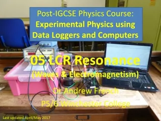
Post-IGCSE Physics Course:Experimental Physics using Data Loggers and Computers05 LCR Resonance (Waves & Electromagnetism) Dr Andrew French P5/6 Winchester College Last updated April/May 2017
Experimental setup Sine wave voltage generator (688.2Hz currently) Windows PC running PicoScope software Picoscope USB oscilloscope A B Resistor (about 380W) 1.0H inductor 0.01 to 0.1mF capacitor A – Voltage across signal generator B – Voltage across terminals of capacitor
An LCR circuit is a single current loop which consists of an Inductor (essentially a coil of wire), a Capacitor (plates to store charge separated by an insulator) and a fixed resistor. Inductor Capacitor ‘driving’ AC input Resistor If an AC source drives current through the circuit, resonant effects can be observed. Around the resonant frequency the voltage response across the capacitor will have a greater amplitude than the driving voltage. The phase of Vc will also vary with driving frequency.
Set timebase Sig gen voltage Vo Set voltage scales Capacitor voltage Vc Useful diagnostic measurements (add via this button) time /ms Set Trigger to be Auto, on source A (i.e. signal generator) Screenshot from PicoScope
Experimental procedure Once Picoscope has been set up and both traces visible clearly, sweep the frequency over an appropriate range and then take screenshots (ctrl+alt+print screen) and paste into IrfanView. Save a PNG bitmap image file with a filename which records the current frequency. e.g. 123p4 Hz.png means ‘100.1 Hz’. A screenshot every 100Hz might be a sensible first move for L = 1.0H and C = 0.07mF, since .... Then more screenshots around the resonance peak might be a good idea (i.e. every 20Hz instead of 100Hz) The resonance frequency is fairly weakly dependent upon resistance, but the peak amplitude will change significantly with the value chosen. The goal of the experiment is to plot Vc amplitude and phase vs frequency for a variety of capacitances, so setting the resistor so that the resonance is ‘sharp enough to observe, but perhaps not too sharp to measure’ is the key idea. Turn the resistor knob and observe the effect near resonance. We need to measure resistance R to fit a model curve. Use a multimeter to achieve this.
186.4 Hz 401.4 Hz PicoScope screenshots Note Vc scale is 5V whereas Vo scale is 2V So they are the same here! L = 1.0H C = 0.07mF 702.9Hz 601.9Hz Clear amplitude gain near resonance, and 90o phase shift 1301Hz 1001Hz About a 180o phase shift well beyond resonance
For phase measurements, drag a box in IrfanView between trough and peak of the V0 trace. Record number of pixels for 180o of phase (look in the title bar). Then work out pixel difference between corresponding peaks or troughs of Vc and Vo traces. Divide both numbers by each other and multiply by 180o 690 pixels 321 pixels 307 pixels For amplitude measurements, simply halve the ‘Peak-to Peak’ values for each trace
Data from Excel sheet overlaid upon a model curve. Computations and graphics production done via a MATLAB program lcr.m More data is needed in the vicinity of the resonance (i.e. in this case between 500Hz and 700Hz)
Data from Excel sheet overlaid upon a model curve. Computations and graphics production done via a MATLAB program lcr.m Note it is harder to make an accurate phase measurement! More data is needed in the vicinity of the resonance
MATLAB code lcr.m i.e. complex impedance potential divider idea
Steady state solution to the LCR circuit Let current I flow through the circuit. The net EMF V - VL must equal the sum of the potential drops across each electrical component. Sum of potential differences EMF – ‘back EMF’ due to induction in the coil Inductor Capacitor ‘driving’ AC input Resistor Steady state solution to SHM equation
Steady state solution to the LCR circuit .... cont Inductor Capacitor ‘driving’ AC input Resistor Steady state solution to SHM equation
Using dimensionless variables ... Note is the average current when the maximum amount of charge stored in the capacitor is discharged over one complete period at frequency f0
Complex impedance Let current I flow through the circuit. The net EMF V - VL must equal the sum of the potential drops across each electrical component. Sum of potential differences EMF – ‘back EMF’ due to induction in the coil Inductor Capacitor ‘driving’ AC input Resistor Inductor Capacitor ‘driving’ AC input Resistor Impedances for L,C,R components Ohm’s Law, generalized for AC
Inductor Resistor ‘driving’ AC input Capacitor