BFS and DFS
830 likes | 1.09k Views
BFS and DFS. BFS and DFS in directed graphs BFS in undirected graphs An improved undirected BFS-algorithm. The Buffered Repository Tree (BRT). Stores key-value pairs (k,v) Supported operations: I NSERT (k,v) inserts a new pair (k,v) into T E XTRACT (k) extracts all pairs with key k

BFS and DFS
E N D
Presentation Transcript
BFS and DFS BFS and DFS in directed graphs BFS in undirected graphs An improved undirected BFS-algorithm
The Buffered Repository Tree (BRT) • Stores key-value pairs (k,v) • Supported operations: • INSERT(k,v) inserts a new pair (k,v) into T • EXTRACT(k) extracts all pairs with key k • Complexity: • INSERT: O((1/B)log2(N/B)) amortized • EXTRACT: O(log2(N/B) + K/B) amortized (K = number of reported elements)
Main memory Disk The Buffered Repository Tree (BRT) • (2,4)-tree • Leaves store between B/4 and B elements • Internal nodes have buffers of size B • Root in main memory, rest on disk
Main memory Main memory Disk Disk INSERT(k,v) • O(X/B) I/Os to empty buffer of size X B • Amortized charge per element and level: O(1/B) • Height of tree: O(log2(N/B)) • Insertion cost: O((1/B)log2(N/B)) amortized
Main memory Main memory Disk Disk EXTRACT(k) • Number of traversed nodes: O(log2(N/B) + K/B) • I/Os per node: O(1) • Cost of operation: O(log2(N/B) + K/B) • But careful with removal of extracted elements Elements with key k
Cost of Rebalancing • O(N/B) leaf creations and deletions • O(N/B) node splits, fusions, merges • Each such operation costs O(1) I/Os • O(N/B) I/Os for rebalancing Theorem:The BRT supports INSERT and EXTRACT operations in O((1/B)log2(N/B)) andO(log2(N/B) + K/B) I/Os amortized.
Directed DFS • Algorithm proceeds as internal memory algorithm: • Use stack to determine order in which vertices are visited • For current vertex v: • Find unvisited out-neighbor w • Push w on the stack • Continue search at w • If no unvisited out-neighbor exists • Remove v from stack • Continue search at v’s parent • Stack operations cost O(N/B) I/Os • Problem: Finding an unvisited vertex
Directed DFS • Data structures: • BRT T • Stores directed edges (v,w) with key v • Priority queues P(v), one per vertex • Stores unexplored out-edges of v • Invariant: Not in P(v) In P(v) and in T In P(v), but not in T
v Directed DFS • Finding next vertex after vertex v: Total:O((|V| + |E|/B)log2(|E|/B)) w EXTRACT(v): Retrieve red edges from T O(|V| log2(|E|/B) + |E|/B) O(log2(|E|/B) + K1/B) Remove these edges from P(v) using DELETE O(|V| + sort(|E|)) O(sort(K1)) Retrieve next edge using DELETEMIN on P(v) O(sort(|E|)) O((1/B)logm(|E|/B)) Insert in-edges of w into T O(1 + (K2/B)log2(|E|/B)) O((|E|/B)log2(|E|/B)) Push w on the stack O(1/B) amortized O(|V|/B)
Directed DFS + BFS • BFS can be solved using same algorithm • Only modification: Use queue (FIFO) instead of stack Theorem:Depth first-search and breadth-first search in a directed graph G = (V,E) can be solved in O((|V|+|E|/B)log2(|E|/B)) I/Os. Exercise: Convince yourself that the priority queues P(v) are not necessary in the case of BFS.
Undirected BFS Observation:For v L(i), all its neighbors are inL(i – 1) L(i) L(i + 1). • Build BFS-tree level by level: • Initially, L(0) = {r} • Given levels L(i – 1) and L(i): • Let X(i) = set of all neighbors of vertices in L(i) • Let L(i + 1) = X(i) \ (L(i – 1) L(i)) Partition graph into levels L(0), L(1), ...around source: L(0), L(1), L(2), L(3)
Undirected BFS Constructing L(i + 1): • Retrieve adjacency lists of vertices in L(i) X(i) • Sort X(i) • Scan L(i – 1), L(i), and X(i) to • Remove duplicates from X(i) • Compute X(i) \ (L(i – 1) L(i)) Complexity: O(|L(i)| + sort(|L(i – 1)| + |X(i)|)) I/Os O( ) I/Os |V| + sort(|E|) Theorem:Breadth-first search in an undirected graph G = (V,E) can be solved in O(|V| + sort(|E|)) I/Os.
A Faster BFS-Algorithm Problem with simple BFS-algorithm: • Random accesses to retrieve adjacency lists Idea for a faster algorithm: • Load more than one adjacency list at a time • Reduces number of random accesses • Causes edges to be involved in more than one iteration of the algorithm • Trade-off
A Faster BFS-Algorithm (Randomized) • Let 0 < m < 1 be a parameter (specified later) • Two phases: • Build m|V| disjoint clusters of diameter O(1/m) • Perform modified version of SIMPLEBFS • Clusters C1,...,Cq formed using BFS from randomly chosen set V’ = {r1,...,rq} of masters • Vertex is chosen as a master with probability m(coin flip) Observation:E[|V’|] = m|V|. That is, the expected number of clusters is m|V|.
Forming Clusters (Randomized) • Apply SIMPLEBFS to form clusters • L(0) = V’ • v Ci if v is descendant of ri s
Forming Clusters (Randomized) Lemma:The expected diameter of a cluster is 2/m. • E[k] 1/m Corollary:The clusters are formed in expected O((1/m)sort(|E|)) I/Os. vk s v5 v4 v3 v2 v1 x
Forming Clusters (Randomized) • Form files F1,...,Fq, one per clusterFi = concatenation of adjacency lists of vertices in Ci • Augment every edge (v,w) Fi with the start position of file Fj s.t. w Cj: • Edge = triple (v,w,pj) s
The BFS-Phase • Maintain a sorted pool H of edges s.t. adjacency lists of vertices in L(i) are contained in H • Scan L(i) and H to find vertices in L(i) whose adjacency lists are not in H • Form list of start positions of files containing these adjacency lists and remove duplicates • Retrieve files, sort them, and merge resulting list H’ with H • Scan L(i) and H to build X(i) • Construct L(i + 1) from L(i – 1), L(i), and X(i) as before O((|L(i)| + |H|)/B) O(sort(|L(i)|)) O(K + sort(|H’|) + |H|/B) O((|L(i)| + |H|)/B) O(sort(|L(i)| + |L(i–1)| + |X(i)|))
The BFS-Phase I/O-complexity of single step: • O(K + |H|/B + sort(|H’| + |L(i – 1)| + |L(i)| + |X(i)|)) • Expected I/O-complexity:O(m|V| + |E|/(mB) + sort(|E|)) • Choose Theorem:BFS in an undirected graph G = (V,E) can be solved in I/Os.
Single Source Shortest Paths The tournament tree SSSP in undirected graphs SSSP in planar graphs
Single Source Shortest Paths • Need: • I/O-efficient priority queue • I/O-efficient method to update only unvisited vertices
The Tournament Tree • I/O-efficient priority queue • Supports: • INSERT(x,p) • DELETE(x) • DELETEMIN • DECREASEKEY(x,p) • All operations take O((1/B)log2(N/B)) I/Os amortized Note:N = size of the universe # elements in the tree
Main memory Disk The Tournament Tree • Static binary tree over all elements in the universe • Elements map to leaves, M elements per leaf • Internal nodes store between M/2 and M elements • Internal nodes have signal buffers of size M • Root in main memory, rest on disk
Main memory Disk The Tournament Tree • Elements stored at each node are sorted by priority • Elements at node v have smaller priority than elements at v’s descendants • Convention: x T if and only if p(x) is finite
v The Tournament TreeDeletions • Operation DELETE(x) signal DELETE(x) x UPDATE(x,) DELETE(x)
v w The Tournament TreeInsertions and Updates • Operations INSERT(x,p) and DECREASEKEY(x,p) signal UPDATE(x,p) x • All elements < p • Forward signal to w • At least one element p • Insert x • Send DELETE(x) to w Current priority p’ If p < p’: Update If p p’: Do nothing
v w The Tournament TreeHandling Overflow • Let y be element with highest priority py • Send signal PUSH(y,py) to appropriate child of v y
v w The Tournament TreeKeeping the Nodes Filled O(M/B) I/Os to move M/2 elements one level up the tree
Main memory Disk The Tournament TreeSignal Propagation • Scan v’s signal, partition into sets Xu and Xw • Load u into memory, apply signals in Xu to u,insert signals into u’s signal buffer • Do the same for w • O((|X| + M)/B) = O(|X|/B) I/Os
The Tournament TreeAnalysis • Elements travel up the tree • Cost: O(1/B) I/Os amortized per element and level • O((K/B)log2(N/B)) I/Os for K operations • Signals travel down the tree • Cost: O(1/B) I/Os amortized per signal and level • O(K) signals for K operations • O((K/B)log2(N/B)) I/Os Theorem:The tournament tree supports INSERT, DELETE, DELETEMIN, and DECREASEKEY operations in O((1/B)log2(N/B)) I/Os amortized.
Single Source Shortest Paths Modified Dijkstra: • Retrieve next vertex v from priority queue Q using DELETEMIN • Retrieve v’s adjacency list • Update distances of all of v’s neighbors, except predecessor u on the path from s to v • Repeat • O(|V| + (E/B)log2(V/B)) I/Os using tournament tree
Single Source Shortest Paths Problem: Observation:If v performs a spurious update of u,u has tried to update v before. • Record this update attempt of u on v by insterting u into another priority queue Q’Priority: d(s,u) + w({u,v}) u v
Single Source Shortest Paths Second modification: • Retrieve next vertex using two DELETEMIN’s,one on Q, one on Q’ • Let (x,px) be the element retrieved from Q,let (y,py) be the element retrieved from Q’ • If px py: re-insert (y,py) into Q’ and proceed as normal • If px < py: re-insert (x,px) into Q and perform a DELETE(y) on Q
Single Source Shortest Paths Lemma:A spurious update is removed from Q before the targeted vertex can be retrieved using DELETEMIN. • Event A: Spurious update happens (“time”: d(s,v)) • Event B: Vertex u is deleted by retrieval of u from Q’ (“time”: d(s,u) + w(e)) • Event C: Vertex u is retrieved from Q using DELETEMIN operation (“time”: d(s,v) + w(e)) u v
Single Source Shortest Paths • Assume that all vertices have different distance from source s • d(u) < d(v) • d(v) d(u) + w(e) < d(u) + w(e) • Sequence of events: A B C Theorem:The single source shortest path problem on an undirected graph G = (V,E) can be solved inO(|V| + (|E|/B)log2(|V|/B)) I/Os.
Planar Graphs Shortest paths in planar graphs Planar separators Planar DFS
GR Shortest Paths in Planar Graphs s
Shortest Paths in Planar Graphs Observation:For every separator vertex v, the distances from s to v in G and GR are the same. • The distances from s to all separator vertices can be computed in GR. s v s v
s Shortest Paths in Planar Graphs Observation:For every vertex v in Gi,dist(s,v) = min{dist(s,x) + dist(x,v) : v Gi}. • Can compute dist(s,v) in the following graph: s v
Shortest Paths in Planar Graphs Three main steps: • Solve all-pairs shortest paths in subgraphs Gi • Compute shortest paths from s to separator vertices in GR • Compute shortest paths from s to all remaining vertices
Shortest Paths in Planar Graphs Regular h-partition: • O(N/h) subgraphs G1,...,Gr • Each Gi has size at most h • Each Gi has boundary size at most • Total number of separator vertices • Number of boundary sets is O(N/h)
Shortest Paths in Planar Graphs Three main steps: • Solve all-pairs shortest paths in subgraphs Gi • Compute shortest paths from s to separator vertices in GR • Compute shortest paths from s to all remaining vertices • Assume the given partition is regular B2-partition • Steps 1 and 3 take O(scan(N)) I/Os • Graph GR has O(N/B) vertices and O(N) edges
Shortest Paths in Planar Graphs Data structures: • List L storing tentative distances of all vertices • Priority queue Q storing vertices with their tentative distances as priorities One step: • Retrieve next vertex v using DELETEMIN • Get distances of v’s neighbors from L • Update their distances in Q using DELETE and INSERT • O(N + sort(N)) I/Os
Shortest Paths in Planar Graphs • One I/O per boundary set • Each boundary set is touched O(B) times: • Once per vertex on the boundary of the region • O(N/B2) boundary sets O(N/B) I/Os
Planar Separator Goal: Compute a separator S of size whose removal partitions G into subgraphs of size at most h. Basic idea: • Compute hierarchy of log(DB) graphs of geometrically decreasing size using graph contraction • Compute a separator of the smallest graph • Undo the contractions and maintain the separator while doing this Assumption: M = W(hlog2 B)
G2 G1 G0 Planar Separator
Planar Separator Properties: • All Gi are planar • |Gi+1| |Gi|/2 • Every vertex in Gi+1 represents only a constant number of vertices in Gi • Every vertex in Gi+1 represents at most 2i+2 vertices in G0 • r = log2(DB) graphs G0,…,Gr • |Gr| = O(N/(DB))
G2 G1 G0 Planar Separator
Planar Separator • Compute separator Sr of Gr: • Sr = Sr partitions Gr into connected components of size at most hlog2(DB) • Takes O(|Gr|) = O(N/B) I/Os [AD96]
Planar Separator • Compute Si from Si+1: • Let Si be the set of vertices in Gi represented by the vertices in Si+1 • Connected components of Gi – Si have size at most chlog2(DB) • Partition every connected components of size more than hlog2(DB) into components of size hlog2(DB)separator Si • Takes O(sort(|Gi|)) I/Os: • Connected components O(sort(|Gi|)) • Partitioning happens in internal memory • Total: O(sort(N)) I/Os