Advanced DFS, BFS, Graph Modeling
Advanced DFS, BFS, Graph Modeling. 19/2/2005. Introduction. Depth-first search (DFS) Breadth-first search (BFS) Graph Modeling Model a graph from a problem, ie. transform a problem into a graph problem. vertex. edge. What is a graph?. A set of vertices and edges. ancestors. root.


Advanced DFS, BFS, Graph Modeling
E N D
Presentation Transcript
Advanced DFS, BFS, Graph Modeling 19/2/2005
Introduction • Depth-first search (DFS) • Breadth-first search (BFS) • Graph Modeling • Model a graph from a problem, ie. transform a problem into a graph problem
vertex edge What is a graph? • A set of vertices and edges
ancestors root parent siblings descendents children Trees and related terms
Graph Traversal • Given: a graph • Goal: visit all (or some) vertices and edges of the graph using some strategy (the order of visit is systematic) • DFS, BFS are examples of graph traversal algorithms • Some shortest path algorithms and spanning tree algorithms have specific visit order
Intuition of DFS of BFS • This is a brief idea of DFS, BFS • DFS: continue visiting next vertex whenever there is a road, go back if no road (ie. visit to the depth of current path) • Example: a human want to visit a place, but do not know the path • BFS: go through all the adjacent vertices before going further (ie. spread among next vertices) • Example: set a house on fire, the fire will spread through the house
DFS (pseudo code) DFS (vertex u) { mark u as visited for each vertex v directly reachable from u if v is unvisited DFS (v) } • Initially all vertices are marked as unvisited
F E unvisited visited A D B C DFS (Demonstration)
“Advanced” DFS • Apart from just visiting the vertices, DFS can also provide us with valuable information • DFS can be enhanced by introducing: • birth time and death time of a vertex • birth time: when the vertex is first visited • death time: when we retreat from the vertex • DFS tree • parent of a vertex
DFS spanning tree / forest • A rooted tree • The root is the start vertex • If v is first visited from u, then u is the parent of v in the DFS tree • Edges are those in forward direction of DFS, ie. when visiting vertices that are not visited before • If some vertices are not reachable from the start vertex, those vertices will form other spanning trees (1 or more) • The collection of the trees are called forest
DFS (pseudo code) DFS (vertex u) { mark u as visited time time+1 for each vertex v directly reachable from u if v is unvisited DFS (v) time time+1 }
A D B E G E F C A D H F unvisited B visited visited (dead) C G H DFS forest (Demonstration) 1 2 3 13 10 4 14 6 12 9 8 16 11 5 15 7 - A B - A C D C
A D B E G C F H Classification of edges • Tree edge • Forward edge • Back edge • Cross edge • Question: which type of edges is always absent in an undirected graph?
Determination of edge types • How to determine the type of an arbitrary edge (u, v) after DFS? • Tree edge • parent [v] = u • Forward edge • not a tree edge; and • birth [v] > birth [u]; and • death [v] < death [u] • How about back edge and cross edge?
Applications of DFS Forests • Topological sorting (Tsort) • Strongly-connected components (SCC) • Some more “advanced” algorithms
Example: Tsort • Topological order: A numbering of the vertices of a directed acyclic graph such that every edge from a vertex numbered i to a vertex numbered j satisfies i<j • Tsort: Number the vertices in topological order 3 6 1 7 2 5 4
Tsort Algorithm • If the graph has more then one vertex that has indegree 0, add a vertice to connect to all indegree-0 vertices • Let the indegree 0 vertice be s • Use s as start vertice, and compute the DFS forest • The death time of the vertices represent the reverse of topological order
A B C G S D F E G C F B A E D D E A B F C G
Example: SCC • A graph is strongly-connected if • for any pair of vertices u and v, one can go from u to v and from v to u. • Informally speaking, an SCC of a graph is a subset of vertices that • forms a strongly-connected subgraph • does not form a strongly-connected subgraph with the addition of any new vertex
SCC (Algorithm) • Compute the DFS forest of the graph G to get the death time of the vertices • Reverse all edges in G to form G’ • Compute a DFS forest of G’, but always choose the vertex with the latest death time when choosing the root for a new tree • The SCCs of G are the DFS trees in the DFS forest of G’
F A D B C G H SCC (Demonstration) 1 2 3 13 10 4 14 6 12 9 8 16 11 5 15 7 - A B - A C D C E F A E B H D A D G F B C C G H
A E B H E D F G F C A D B C G H SCC (Demonstration)
DFS Summary • DFS spanning tree / forest • We can use birth time and death time in DFS spanning tree to do varies things, such as Tsort, SCC • Notice that in the previous slides, we related birth time and death time. But in the discussed applications, birth time and death time can be independent, ie. birth time and death time can use different time counter
DFS (vertex u) { mark u as visited birthtime birthtime + 1 for each vertex v directly reachable from u if v is unvisited DFS (v) deathtime deathtime + 1 } time time+1 time time+1
Breadth-first search (BFS) • Revised: • DFS: continue visiting next vertex whenever there is a road, go back if no road (ie. visit to the depth of current path) • BFS: go through all the adjacent vertices before going further (ie. spread among next vertices) • In order to “spread”, we need to makes use of a data structure, queue ,to remember just visited vertices
BFS (Pseudo code) while queue not empty dequeue the first vertex u from queue for each vertex v directly reachable from u if v is unvisited enqueue v to queue mark v as visited • Initially all vertices except the start vertex are marked as unvisited and the queue contains the start vertex only
I G D C H unvisited visited A E J visited (dequeued) F B BFS (Demonstration) Queue: A B C F D E H G J I
Applications of BFS • Shortest paths finding • Flood-fill (can also be handled by DFS)
start goal Bidirectional search (BDS) • Searches simultaneously from both the start vertex and goal vertex • Commonly implemented as bidirectional BFS
BDS Example: Bomber Man (1 Bomb) • find the shortest path from the upper-left corner to the lower-right corner in a maze using a bomb. The bomb can destroy a wall.
Bomber Man (1 Bomb) 1 2 3 4 13 12 11 12 4 10 7 6 6 7 8 9 8 5 9 5 4 3 2 1 10 11 12 13 Shortest Path length = 7 What will happen if we stop once we find a path?
Iterative deepening search (IDS) • Iteratively performs DFS with increasing depth bound • Shortest paths are guaranteed
IDS (pseudo code) DFS (vertex u, depth d) { mark u as visited if (d>0) for each vertex v directly reachable from u if v is unvisited DFS (v,d-1) } i=0 Do { DFS(start vertex,i) Increment i }While (target is not found)
IDS Complexity(the details can be skipped) • ( )=bm • ( ) =bm - b is branching factor- td is the number of vertices visited for depth d
IDS • ( )=bm • ( ) =bm - b is branching factor- td is the number of vertices visited for depth d • Conclusion: the complexity of IDS is the same as DFS
Summary of DFS, BFS • We learned some variations of DFS and BFS • Bidirectional search (BDS) • Iterative deepening search (IDS)
What is graph modeling? • Conversion of a problem into a graph problem • Sometimes a problem can be easily solved once its underlying graph model is recognized • Graph modeling appears almost every year in NOI or IOI
Basics of graph modeling • A few steps: • identify the vertices and the edges • identify the objective of the problem • state the objective in graph terms • implementation: • construct the graph from the input instance • run the suitable graph algorithms on the graph • convert the output to the required format
start goal Simple examples (1) • Given a grid maze with obstacles, find a shortest path between two given points
Simple examples (2) • A student has the phone numbers of some other students • Suppose you know all pairs (A, B) such that A has B’s number • Now you want to know Alan’s number, what is the minimum number of calls you need to make?
Simple examples (2) • Vertex: student • Edge: whether A has B’s number • Add an edge from A to B if A has B’s number • Problem: find a shortest path from your vertex to Alan’s vertex
Complex examples (1) • Same settings as simple example 1 • You know a trick – walking through an obstacle! However, it can be used for only once (Bomber Man with 1 bomb) • What should a vertex represent? • your position only? • your position + whether you have used the trick
Complex examples (1) • A vertex is in the form (position, used) • The vertices are divided into two groups • trick used • trick not used
start goal Complex examples (1) unused start goal used goal
Complex examples (1) • How about you can walk through obstacles for k times?