ARSM -ASFM reduction

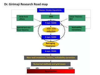
1. Navier-Stokes Equations DNS Body force effects Linear Theories: RDT 7-eqn. RANS Realizability, Consistency Spectral and non-linear theories ARSM -ASFM reduction 2-eqn. RANS Averaging Invariance 2-eqn. PANS Near-wall treatment, limiters, realizability correction Numerical methods and grid issues Application Dr. Girimaji Research Road map DNS LES RANS

2. Objective • Need for a new approach to modeling the scalar flux considering compressibility effects Mg effect • Application: Turbulent combustion/mixing in hypersonic aircrafts • Physical sequence of mixing: Turbulent Stirring Molecular Mixing Chemical Reaction

3. Turbulent mixing Velocity Field (ARSM), Scalar Dissipation Rate, Turbulent Stirring Molecular Mixing Chemical Reaction [Gaurav] [Carlos] Scalar Flux Field (ASFM), [Mona]

4. Scalar Flux molding approaches Modeling Differential Transport eq. Constitutive Relations Weak Equilibrium assumption Representation theory Reduced Differential algebraic

5. Algebraic Scalar Flux modeling approach: ARSM: Weak equilibrium assumption ASFM with variable Pr_teffect

6. Algebraic Scalar Flux modeling approach (step-by-step) Step (1) the evolution of passive scalar flux • Step (2) Assumptions: • the isotropy of small scales • weak equilibrium condition, advection and diffusion terms  0 Step (3) Pressure –scalar gradient correlation

7. Algebraic Scalar Flux modeling approach (step-by-step) Step (3) Modeling Pressure-scalar gradient correlation High Mg- pressure effect is negligible. Intermediate Mg - pressure nullifies inertial effects. Low Mg – Incompressible limit [Craft & Launder, 1996] Step (4) Applying ARSM by Girimaji’s group

8. Algebraic Scalar Flux modeling approach (step-by-step) Step (4) using ARSM developed by Girimaji group, [Wikström et al, 2000] : = Tensorial eddy diffusivity

9. Preliminary Validation of the Model Standard k-ε model 1-a) with constant- Cμ =0.09 1-b) variable- Cμ with Mg effects which uses the linear ARSM [Gomez & Girimaji ] Assume Pr_t = 0.85 Variable tensorial diffusivity

10. Geometry of planar mixing layer Isentropic relations (compressible flows) 0.025 Fast stream Tt1 = 295 K, M=2.01 Pressure inlet slow stream Tt2 = 295 K, M=1.38 Pressure inlet - 0.025 X=0 X=0.5 X=0.1 X=0.15 X=0.2 X=0.25 X=0.3 y x for both free-stream inlets the turbulent intensity =0.01 %, turbulent viscosity ratio = 0.1

11. Schematic of planar mixing layer U1 M1 T1 Pressure-inlet Ptot,1 Pstat,1 Pressure-outlet Tout NRBC: avg bd. press. Fast stream Slow stream Pressure-inlet Ptot,1 Pstat,1 U2 M2 T1

12. Post-processing • Normalized mean total temperature The mean total temperature is normalized by initial mean temperature difference of two streams and cold stream temperature. Due to the Boundedness of the totaltemperature, the normalized value, in theory, should remain between zero and unity. • Eddy diffusivity (eddy diffusion coefficient) For the approach (a), in which the turbulence model is the standard k-ε, the scalar diffusion on coefficient or eddy diffusivity is obtained by modeling the turbulent scalar transport using the concept of “Reynolds’ analogy” to turbulent momentum transfer. Thus, the modeled energy equation is given by

13. Post-processing • Flux components • Constant-/variable-Cμ • Tensorial eddy diffusivity • Streamwisescalar flux: • Transversal scalar flux:. • Thickness growth rate [ongoing]

14. 1-a) Standard k-ε model with constant-Cμ

15. Normalized Temp Contours Case -5Mr = 1.97 1-a) Standard k-ε model with constant-Cμ Case -2Mr = 0.91 Case -3rMr = 1.44 Case -4Mr = 1.73

16. Case -5Mr = 1.97 Bounded Normalized Temp Contours Case -2Mr = 0.91 Case -3rMr = 1.44 Case -4Mr = 1.73

17. Fast stream Slow stream Normalized Temp Profile 1-a) Standard k-ε model with constant-Cμ

18. Fast stream Slow stream Eddy diffusivity profile 1-a) Standard k-ε model with constant-Cμ

19. Scalar flux components 1-a) Standard k-ε model with constant-Cμ Streamwise scalar flux @ x=0.2 Fast stream Slow stream

20. Scalar flux components 1-a) Standard k-ε model with constant-Cμ Transversal scalar flux @ x=0.2 Fast stream Slow stream

21. Eddy diffusivity profile for case 5 (Mr=1.97), @ different stations Toward outlet Fast stream Slow stream

22. 1-a) Standard k-ε model with constant-Cμ Comparing Scalar flux components, Axial vs. Transversal for Mr-1.8 (case5) and Mr 0.97 (case2)

23. 1-b) Standard k-ε model with variable Cμ (Mg effect)

24. Normalized Total Temp Profile @ x=0.02 Fast stream Slow stream 1-a) Standard k-ε model with constant-Cμ 1-b) Standard k-ε model with variable Cμ (Mg effect)

25. Eddy Diffusivity Profile @ x=0.02 1-a) Standard k-ε model with constant-Cμ 1-b) Standard k-ε model with variable Cμ (Mg effect)

26. Streamwise scalar flux @ x=0.02 1-a) Standard k-ε model with constant-Cμ 1-b) Standard k-ε model with variable Cμ (Mg effect)

27. Transversal scalar flux @ x=0.02 1-a) Standard k-ε model with constant-Cμ 1-b) Standard k-ε model with variable Cμ (Mg effect)

28. Convergence issues • All simulations were continued until a self-similar profiles (for mean velocity and temperature) are achieved in different Mach cases. • Main Criterion to check convergence : imbalance of Flux (Mass flow rate ) across the boundaries (inlet & outlet) goes to zero. < 0.2% • Error-function profile  self-similarity state • Normalized mean stream-wise velocity • Normalized mean temperature