Algorithm Driven Fluid Simulation
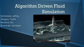
Algorithm Driven Fluid Simulation. Dombroski, Jeffrey Gregory, Taylor Rackear, Eric Shotande, Monique. Overview. Main methods to model fluids Eulerian (grid) Lagrangian (particles). Navier-Stokes Equation Advection Velocity Density Pressure Viscosity Time External forces.

Algorithm Driven Fluid Simulation
E N D
Presentation Transcript
Algorithm Driven Fluid Simulation Dombroski, Jeffrey Gregory, Taylor Rackear, Eric Shotande, Monique
Main methods to model fluids Eulerian (grid) Lagrangian (particles)
Navier-Stokes Equation Advection Velocity Density Pressure Viscosity Time External forces
Typical Simulations Water drop Broken dam
Particle-In-Cell (PIC) method Focuses on manipulated particles’ centers, represented by a small mass This allows transient and compressible flow of multiple materials with no restrictions
Particle variables Position, Mass, Species information (for placement on Eulerian 2D mesh)
Particle variables • Position, • Mass, • Species information (for placement on Eulerian 2D mesh)
Marker and Cell (MAC) Developed in 1965 by Francis Harlow and the TI-3 group at the Los Alamos National Laboratory
Built upon the PIC method • First successful technique that allowed incompressible fluids to flow without too much distortion • Calculations do not need to be “reset” by hand, unlike PIC • Particles used as markers to locate mesh material
2 Dimensional View of the grid Schematic view of the two-dimensional MAC mesh. •, ϕ and Π nodes; ○;, ϕ and Π boundary nodes; □, Ux nodes; and ◊, Uynodes
Problems with the MAC method The original MAC method tracked every single cell in the grid, although most of the cells were empty At the time, computers struggled with this level of computation and there were stability issues related to the centering of the momentum for each particle This instability was identified in 1968 and the issue was related to running simulations with too low of a viscosity
A single MAC Cell Harlow and Welch stabilized the simulations by centering each velocity component on a face of the cell instead of calculating all three at the center
Modern Use of the MAC Method In this use of the MAC method, cells are dynamically created and destroyed in order to minimize the amount of computations needed to be made These particles are rendered as 2-Dimensional circles instead of spheres. For the final version of the simulation, the particles are rendered as spheres instead
Most widespread method Fluid divided into a set of particles Each with a spatial distance, called the smoothing length
Kernel function smooths these properties over the smoothing length Physical quantity of particle result of summation of relevant properties of particles within kernel range Kernel, common functions: Gaussian function Cubic spline
Cubic spline Zero for particles 2+ smoothing lengths away Computational advantage through exclusion of insignificant effects from distant particles Gaussian function Particles contribute no matter the distance
where Mj is the mass of particle j, Aj is the value of the quantity A for particle j, Pj is the density associated with particle j, r is the position and W is the kernel functionImplementation1. Initiate by defining particle attributes that include mass, position, and density for each particle.2. Set up the particles in either a 2D or 3D space using either a Cartesian grid or cubic lattice respectively. Using a 3D space is preferred as it has a higher accuracy than a 2D grid system.3. For a number of repetitions, calculate A(r) for each particle. This can be done using a time-step equation that will ensure conservation of energy.
AdvantagesDoesn't use a grid to solve systems of linear equations Instead finds particle information by using weighted neighboring particle information Can be used in real time simulation because fluid boundaries don't need to be tracked
DisadvantagesUnable to produce quality resolution simulations equal to grid systems To do this requires a large number of particles (becomes too computationally expensive)Problem to solve: enforcing incompressibility(constant density of particle) which is essential for realism
ApplicationsOften used in games and real time animations where interactivity with the fluid is more important than realism and highly accurate simulations
Advances in IncompressibilityNew models of method apply constraints enforcing constant density on par which grid based systems Big step up in efficiency, still not good enough for real time applications of highly realistic simulations
LBM Pro: Fast Con: requires large amount of memory Streaming step Collision step PLSM Visually detailed Computational expensive
The Algorithm 1. Execute LBM solver 2. Calculate velocities 3. Execute PLSM solver 4. Advect level set function 5. Correct errs from level set functions 6. Calculate density fields from the LBM and PLSM solvers 7. Add density difference to distribution functions to correct LBM errors