Download

1 / 16
160 likes | 301 Views
Latent Semantic Indexing (mapping onto a smaller space of latent concepts). Paolo Ferragina Dipartimento di Informatica Università di Pisa. Reading 18. Speeding up cosine computation.

E N D
Latent Semantic Indexing(mapping onto a smaller space of latent concepts) Paolo Ferragina Dipartimento di Informatica Università di Pisa Reading 18
Speeding up cosine computation • What if we could take our vectors and “pack” them into fewer dimensions (say 50,000100) while preserving distances? • Now, O(nm) to compute cos(d,q) for all d • Then, O(km+kn) where k << n,m • Two methods: • “Latent semantic indexing” • Random projection
Briefly • LSI is data-dependent • Create a k-dim subspace by eliminating redundant axes • Pull together “related” axes – hopefully • car and automobile • Random projection is data-independent • Choose a k-dim subspace that guarantees good stretching properties with high probability between any pair of points. What about polysemy ?
Notions from linear algebra • Matrix A, vector v • Matrix transpose (At) • Matrix product • Rank • Eigenvalues l and eigenvector v: Av = lv
Overview of LSI • Pre-process docs using a technique from linear algebra called Singular Value Decomposition • Create a new (smaller) vector space • Queries handled (faster) in this new space
Singular-Value Decomposition • Recall mn matrix of terms docs, A. • A has rank r m,n • Define term-term correlation matrix T=AAt • T is a square, symmetric mm matrix • Let P be mrmatrix of eigenvectors of T • Define doc-doc correlation matrix D=AtA • D is a square, symmetric nn matrix • Let R be nrmatrix of eigenvectors of D
A’s decomposition • Given P(for T, mr) and R(for D, nr) formed by orthonormal columns (unit dot-product) • It turns out that A = PSRt • WhereS is a diagonal matrix with the eigenvalues of T=AAt in decreasing order. mn mr rn = rr Rt S P A
document k k 0 k 0 0 useless due to 0-col/0-row of Sk Dimensionality reduction • For some k << r, zeroout all but the k biggest eigenvalues in S[choice of k is crucial] • Denote by Sk this new version of S, having rank k • Typically k is about 100, while r (A’s rank) is > 10,000 = r Sk Rt S P A Ak k x n r x n m x r m x k
Guarantee • Akis a pretty good approximation to A: • Relative distances are (approximately) preserved • Of all mn matrices of rank k, Ak is the best approximation to A wrt the following measures: • minB, rank(B)=k ||A-B||2 = ||A-Ak||2 = sk+1 • minB, rank(B)=k ||A-B||F2 = ||A-Ak||F2 = sk+12+ sk+22+...+ sr2 • Frobenius norm ||A||F2 = s12+ s22+...+ sr2
R,P are formed by orthonormal eigenvectors of the matrices D,T Reduction • Xk = Sk Rtis the doc-matrix k x n, hence reduced to k dim • Since we are interested in doc/q-correlation, we consider: • D=AtA=(P SRt)t(P SRt) = (SRt)t (SRt) • Approx S with Sk, thus get AtA Xkt Xk (both are n x n matr.) • We use Xkto define how to project A and Q: • Xk= SkRt , substitute Rt = S-1Pt A, so getPkt A. • In fact, SkS-1Pt = Pkt which is a k x m matrix • This means that to reduce a doc/query vector is enough to multiply it by Pkt thus paying O(km) per doc/query • Cost of sim(q,d), for all d, is O(kn+km) instead of O(mn)
Which are the concepts ? • c-th concept = c-th row of Pkt (which is k x m) • Denote it by Pkt [c], whose size is m = #terms • Pkt [c][i] = strength of association between c-th concept and i-th term • Projected document: d’j= Pkt dj • d’j[c] = strenght of concept c in dj • Projected query: q’= Pkt q • q’[c] = strenght of concept c in q
Random Projections Paolo Ferragina Dipartimento di Informatica Università di Pisa Slides only !
An interesting math result Lemma (Johnson-Linderstrauss, ‘82) Let P be a set of n distinct points in m-dimensions. Given e > 0, there exists a function f : P IRk such that for every pair of points u,v in P it holds: (1 - e) ||u - v||2 ≤ ||f(u) – f(v)||2 ≤(1 + e) ||u-v||2 Where k = O(e-2 log m) f() is called JL-embedding Setting v=0 we also get a bound on f(u)’s stretching!!!
What about the cosine-distance ? f(u)’s, f(v)’s stretching substituting formula above for ||u-v||2
E[ri,j] = 0 Var[ri,j] = 1 How to compute a JL-embedding? If we set R = ri,j to be a random mx k matrix, where the components are independent random variables with one of the following distributions
Finally... • Random projections hide large constants • k (1/e)2 * log m, so it may be large… • it is simple and fast to compute • LSI is intuitive and may scale to any k • optimal under various metrics • but costly to compute