Download
1 / 49
490 likes | 671 Views
Latent Semantic Indexing SI650: Information Retrieva l. Winter 2010 School of Information University of Michigan. … Latent semantic indexing Singular value decomposition …. Problems with lexical semantics. Polysemy bar , bank, jaguar, hot tend to reduce precision Synonymy

E N D
Latent Semantic IndexingSI650: Information Retrieval Winter 2010 School of Information University of Michigan
… Latent semantic indexing Singular value decomposition …
Problems with lexical semantics • Polysemy • bar, bank, jaguar, hot • tend to reduce precision • Synonymy • building/edifice, Large/big, Spicy/hot • tend to reduce recall • Relatedness • doctor/patient/nurse/treatment • Sparse matrix • Need: dimensionality reduction
Problem in Retrieval Query = “information retrieval” Document 1 = “inverted index precision recall” Document 2 = “welcome to ann arbor” • Which one should we rank higher? • Query vocabulary & doc vocabulary mismatch! • Smoothing won’t help here… • If only we can represent documents/queries by topics!
Latent Semantic Indexing • Motivation • Query vocabulary & doc vocabulary mismatch • Need to match/index based on concepts (or topics) • Main idea: • Projects queries and documents into a space with “latent” semantic dimensions • Dimensionality reduction: the latent semantic space has fewer dimensions (semantic concepts) • Exploits co-occurrence: Co-occurring terms are projected onto the same dimensions
Example of “Semantic Concepts” (Slide from C. Faloutsos’s talk)
Concept Space = Dimension Reduction • Number of concepts (K) is always smaller than the number of words (N) or number of documents (M). • If we represent a document as a N-dimension vector; and the corpus as an M*N matrix… • The goal is to reduce the dimension from N to K. • But how can we do that?
Techniques for dimensionality reduction • Based on matrix decomposition (goal: preserve clusters, explain away variance) • A quick review of matrices • Vectors • Matrices • Matrix multiplication
Eigenvectors and eigenvalues • An eigenvector is an implicit “direction” for a matrix where v (eigenvector)is non-zero, though λ (eigenvalue) can be any complex number in principle • Computing eigenvalues (det = determinant): if A is square (N x N), has r distinct solutions, where 1 <= r <= N • For each λ found, you can find v by , or
Eigenvectors and eigenvalues • Example: • det (A-lI) = (-1-l)*(-l)-3*2=0 • Then: l+l2-6=0; l1=2; l2=-3 • For l1=2: • Solutions: x1=x2
Eigenvectors and eigenvalues Wait, that means there are many eigenvectors for the same eigenvalue… v = (x1, x2)T; x1 = x2 corresponds to many vectors, e.g., (1, 1)T, (2, 2)T, (650, 650)T… Not surprising … if v is an eigenvector of A, v’ = cv is also an eigenvector (c is any non-zero constant)
Matrix Decomposition • If A is a square (N x N) matrix and it has N linearly independent eigenvectors, it can be decomposed into ULU-1 where U: matrix of eigenvectors (every column) L: diagonal matrix of eigenvalues • AU = UL • U-1AU = L • A = ULU-1
Example Eigenvaluesare 3, 2, 0 x is an arbitrary vector, yet Sx depends on the eigenvalues and eigenvectors
What about an arbitrary matrix? • A: n x m matrix (n documents, m terms) • A = USVT (as opposed to A = ULU-1) • U: n x n matrix; • V: m x m matrix • S: n x m diagonal matrix only values on the diagonal can be non-zero. • UUT = I; VVT = I
SVD: Singular Value Decomposition • A=USVT • U is the matrix of orthogonal eigenvectors of AAT • V is the matrix of orthogonal eigenvectors of ATA • The components of S are the eigenvalues of ATA • This decomposition exists for all matrices, dense or sparse • If A has 5 columns and 3 rows, then U will be 5x5 and V will be 3x3 • In Matlab, use [U,S,V] = svd (A)
Term matrix normalization D1 D2 D3 D4 D5 D1 D2 D3 D4 D5
Example (Berry and Browne) • T1: baby • T2: child • T3: guide • T4: health • T5: home • T6: infant • T7: proofing • T8: safety • T9: toddler • D1: infant & toddler first aid • D2: babies & children’s room (for your home) • D3: childsafety at home • D4: your baby’s health and safety: from infant to toddler • D5: babyproofing basics • D6: your guide to easy rust proofing • D7: beanie babies collector’s guide
Decomposition u = -0.6976 -0.0945 0.0174 -0.6950 0.0000 0.0153 0.1442 -0.0000 0 -0.2622 0.2946 0.4693 0.1968 -0.0000 -0.2467 -0.1571 -0.6356 0.3098 -0.3519 -0.4495 -0.1026 0.4014 0.7071 -0.0065 -0.0493 -0.0000 0.0000 -0.1127 0.1416 -0.1478 -0.0734 0.0000 0.4842 -0.8400 0.0000 -0.0000 -0.2622 0.2946 0.4693 0.1968 0.0000 -0.2467 -0.1571 0.6356 -0.3098 -0.1883 0.3756 -0.5035 0.1273 -0.0000 -0.2293 0.0339 -0.3098 -0.6356 -0.3519 -0.4495 -0.1026 0.4014 -0.7071 -0.0065 -0.0493 0.0000 -0.0000 -0.2112 0.3334 0.0962 0.2819 -0.0000 0.7338 0.4659 -0.0000 0.0000 -0.1883 0.3756 -0.5035 0.1273 -0.0000 -0.2293 0.0339 0.3098 0.6356 v = -0.1687 0.4192 -0.5986 0.2261 0 -0.5720 0.2433 -0.4472 0.2255 0.4641 -0.2187 0.0000 -0.4871 -0.4987 -0.2692 0.4206 0.5024 0.4900 -0.0000 0.2450 0.4451 -0.3970 0.4003 -0.3923 -0.1305 0 0.6124 -0.3690 -0.4702 -0.3037 -0.0507 -0.2607 -0.7071 0.0110 0.3407 -0.3153 -0.5018 -0.1220 0.7128 -0.0000 -0.0162 -0.3544 -0.4702 -0.3037 -0.0507 -0.2607 0.7071 0.0110 0.3407
Decomposition Spread on the v1 axis S = 1.5849 0 0 0 0 0 0 0 1.2721 0 0 0 0 0 0 0 1.1946 0 0 0 0 0 0 0 0.7996 0 0 0 0 0 0 0 0.7100 0 0 0 0 0 0 0 0.5692 0 0 0 0 0 0 0 0.1977 0 0 0 0 0 0 0 0 0 0 0 0 0 0
What does this have to do with dimension reduction? Low rank matrix approximation SVD: A[m*n] = U[m*m]S[m*n]VT[n*n] Remember that S is a diagonal matrix of eigenvalues If we only keep the largest r eigenvalues.. A ≈ U[m*r]S[r*r]VT[n*r]
Rank-4 approximation s4 = 1.5849 0 0 0 0 0 0 0 1.2721 0 0 0 0 0 0 0 1.1946 0 0 0 0 0 0 0 0.7996 0 0 0 0 0 0 0 0 0 0 0 0 0 0 0 0 0 0 0 0 0 0 0 0 0 0 0 0 0 0 0 0 0 0 0 0 0 0
Rank-4 approximation u*s4*v' -0.0019 0.5985 -0.0148 0.4552 0.7002 0.0102 0.7002 -0.0728 0.4961 0.6282 0.0745 0.0121 -0.0133 0.0121 0.0003 -0.0067 0.0052 -0.0013 0.3584 0.7065 0.3584 0.1980 0.0514 0.0064 0.2199 0.0535 -0.0544 0.0535 -0.0728 0.4961 0.6282 0.0745 0.0121 -0.0133 0.0121 0.6337 -0.0602 0.0290 0.5324 -0.0008 0.0003 -0.0008 0.0003 -0.0067 0.0052 -0.0013 0.3584 0.7065 0.3584 0.2165 0.2494 0.4367 0.2282 -0.0360 0.0394 -0.0360 0.6337 -0.0602 0.0290 0.5324 -0.0008 0.0003 -0.0008
Rank-4 approximation u*s4: word vector representation of the concepts/topics -1.1056 -0.1203 0.0207 -0.5558 0 0 0 -0.4155 0.3748 0.5606 0.1573 0 0 0 -0.5576 -0.5719 -0.1226 0.3210 0 0 0 -0.1786 0.1801 -0.1765 -0.0587 0 0 0 -0.4155 0.3748 0.5606 0.1573 0 0 0 -0.2984 0.4778 -0.6015 0.1018 0 0 0 -0.5576 -0.5719 -0.1226 0.3210 0 0 0 -0.3348 0.4241 0.1149 0.2255 0 0 0 -0.2984 0.4778 -0.6015 0.1018 0 0 0
Rank-4 approximation s4*v': new (concept/topic) representation of documents -0.2674 -0.7087 -0.4266 -0.6292 -0.7451 -0.4996 -0.7451 0.5333 0.2869 0.5351 0.5092 -0.3863 -0.6384 -0.3863 -0.7150 0.5544 0.6001 -0.4686 -0.0605 -0.1457 -0.0605 0.1808 -0.1749 0.3918 -0.1043 -0.2085 0.5700 -0.2085 0 0 0 0 0 0 0 0 0 0 0 0 0 0 0 0 0 0 0 0 0 0 0 0 0 0 0 0 0 0 0 0 0 0 0
Rank-2 approximation s2 = 1.5849 0 0 0 0 0 0 0 1.2721 0 0 0 0 0 0 0 0 0 0 0 0 0 0 0 0 0 0 0 0 0 0 0 0 0 0 0 0 0 0 0 0 0 0 0 0 0 0 0 0 0 0 0 0 0 0 0 0 0 0 0 0 0 0
Rank-2 approximation u*s2*v' 0.1361 0.4673 0.2470 0.3908 0.5563 0.4089 0.5563 0.2272 0.2703 0.2695 0.3150 0.0815 -0.0571 0.0815 -0.1457 0.1204 -0.0904 -0.0075 0.4358 0.4628 0.4358 0.1057 0.1205 0.1239 0.1430 0.0293 -0.0341 0.0293 0.2272 0.2703 0.2695 0.3150 0.0815 -0.0571 0.0815 0.2507 0.2412 0.2813 0.3097 -0.0048 -0.1457 -0.0048 -0.1457 0.1204 -0.0904 -0.0075 0.4358 0.4628 0.4358 0.2343 0.2454 0.2685 0.3027 0.0286 -0.1073 0.0286 0.2507 0.2412 0.2813 0.3097 -0.0048 -0.1457 -0.0048
Rank-2 approximation u*s2: word vector representation of the concepts/topics -1.1056 -0.1203 0 0 0 0 0 -0.4155 0.3748 0 0 0 0 0 -0.5576 -0.5719 0 0 0 0 0 -0.1786 0.1801 0 0 0 0 0 -0.4155 0.3748 0 0 0 0 0 -0.2984 0.4778 0 0 0 0 0 -0.5576 -0.5719 0 0 0 0 0 -0.3348 0.4241 0 0 0 0 0 -0.2984 0.4778 0 0 0 0 0
Rank-2 approximation s2*v': new (concept/topic) representation of documents -0.2674 -0.7087 -0.4266 -0.6292 -0.7451 -0.4996 -0.7451 0.5333 0.2869 0.5351 0.5092 -0.3863 -0.6384 -0.3863 0 0 0 0 0 0 0 0 0 0 0 0 0 0 0 0 0 0 0 0 0 0 0 0 0 0 0 0 0 0 0 0 0 0 0 0 0 0 0 0 0 0 0 0 0 0 0 0 0
Latent Semantic Indexing A[n x m]≈ U[n x r]L [ r x r] (V[m x r])T • A: n x m matrix (n documents, m terms) • U: n x r matrix (n documents, r concepts) • L: r x r diagonal matrix (strength of each ‘concept’) (r : rank of the matrix) • V: m x r matrix (m terms, r concepts)
Latent semantic indexing (LSI) • Dimensionality reduction = identification of hidden (latent) concepts • Query matching in latent space • LSI matches documents even if they don’t have words in common; • If they share frequently co-occurring terms
Back to the CS-MED example (Slide from C. Faloutsos’s talk)
Example of LSI A = ULVT retrieval CS-concept lung MD-concept inf brain data Strength of CS-concept Dim. Reduction CS x x = MD Term rep of concept (Slide adapted from C. Faloutsos’s talk)
retrieval inf. lung brain data qT= How to Map Query/Doc to the Same Concept Space? qTconcept = qT V dTconcept = dT V CS-concept Similarity with CS-concept = dT= 0 1 1 0 0 1.16 0 (Slide adapted from C. Faloutsos’s talk)
Useful pointers • http://lsa.colorado.edu • http://lsi.research.telcordia.com • http://www.cs.utk.edu/~lsi
Readings • MRS18 • MRS17, MRS19 • MRS20
Problem of LSI Concepts/Topics are hard to interpret New document/query vectors could have negative values Lack of statistical interpretation Probabilistic latent semantic indexing…
General Idea of Probabilistic Topic Models • Modeling a topic/subtopic/theme with a multinomial distribution (unigram LM) • Modeling text data with a mixture model involving multinomial distributions • A document is “generated” by sampling words from some multinomial distribution • Each time, a word may be generated from a different distribution • Many variations of how these multinomial distributions are mixed • Topic mining = Fitting the probabilistic model to text • Answer topic-related questions by computing various kinds of conditional probabilities based on the estimated model (e.g., p(time | topic), p(time | topic, location))
Document as a Sample of Mixed Topics [ Criticism of government response to the hurricane primarily consisted of criticism of its response to the approach of the storm and its aftermath, specifically in the delayed response ] to the [flooding of New Orleans. … 80% of the 1.3 million residents of the greater New Orleans metropolitan area evacuated ] …[ Over seventy countries pledged monetary donations or other assistance]. … government 0.3 response 0.2... Topic 1 • Applications of topic models: • Summarize themes/aspects • Facilitate navigation/browsing • Retrieve documents • Segment documents • Many others • How can we discover these topic word distributions? city 0.2new 0.1orleans 0.05 ... Topic 2 … donate 0.1relief 0.05help 0.02 ... Topic k is 0.05the 0.04a 0.03 ... Background B
Probabilistic Latent Semantic Analysis/Indexing (PLSA/PLSI) [Hofmann 99] • Mix k multinomial distributions to generate a document • Each document has a potentially different set of mixing weights which captures the topic coverage • When generating words in a document, each word may be generated using a DIFFERENT multinomial distribution (this is in contrast with the document clustering model where, once a multinomial distribution is chosen, all the words in a document would be generated using the same model) • We may add a background distribution to “attract” background words
PLSI (a.k.a. Aspect Model) • Every document is a mixture of underlying (latent) K aspects (topics) with mixture weights p(z|d) • How is this related to LSI? • Each aspect is represented by a distribution of words p(w|z) • Estimate p(z|d) and p(w|z) using EM algorithm
PLSI as a Mixture Model Document d warning 0.3 system 0.2.. ? Topic z1 ? p(z1|d) 1 “Generating” word w in doc d in the collection 2 aid 0.1donation 0.05support 0.02 .. ? Topic z2 1 - B ? p(z2|d) ? p(zk|d) W k … statistics 0.2loss 0.1dead 0.05 .. ? B ? Topic zk ? B is 0.05the 0.04a 0.03 .. ? ? Background B Parameters: B=noise-level (manually set) P(z|d) and p(w|z) are estimated with Maximum Likelihood ?
Parameter Estimation using EM Algorithm • We have the equation for log-likelihood function from the PLSI model, which we want to maximize: • Maximizing likelihood using Expectation Maximization
EM Steps • E-Step • Expectation step where expectation of the likelihood function is calculated with the current parameter values • M-Step • Update the parameters with the calculated posterior probabilities • Find the parameters that maximizes the likelihood function
E Step • It is the probability that a word w occurring in a document d, is explained by topic z
M Step • All these equations use p(z|d,w) calculated in E Step • Converges to a local maximum of the likelihood function • We will see more when we talk about topic modeling
Topics represented as word distributions - Example of topics found from blog articles about “Hurricane Katrina” Topics are interpretable!