Chapter 6 Introduction to Inference

1. Chapter 6Introduction to Inference

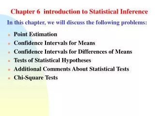
2. Chapter 6Introduction to Inference 6.1 Estimating with Confidence 6.2 Tests of Significance 6.3 Use and Abuse of Tests 6.4 Power and Inference as a Decision

3. 6.1 Estimating with Confidence • Inference • Statistical Confidence • Confidence Intervals • Confidence Interval for a Population Mean • Choosing the Sample Size

4. Statistical Inference After we have selected a sample, we know the responses of the individuals in the sample. However, the reason for taking the sample is to infer from that data some conclusion about the wider population represented by the sample. Statistical inference provides methods for drawing conclusions about a population from sample data. Population Sample Collect data from a representative Sample... Make an Inference about the Population.

5. Simple Conditions for InferenceAbout a Mean This chapter presents the basic reasoning of statistical inference. We start with a setting that is too simple to be realistic. Simple Conditions for Inference About a Mean We have an SRS from the population of interest. There is no nonresponse or other practical difficulty. The variable we measure has an exactly Normal distribution N(μ,σ) in the population. We don’t know the population mean μ, but we do know the population standard deviation σ. Note: The conditions that we have a perfect SRS, that the population is exactly Normal, and that we know the population standard deviation are all unrealistic.

6. Statistical Estimation Suppose your instructor has selected a “Mystery Mean” value µ and stored it as “M” in their calculator. The following command was executed on their calculator: mean(randNorm(M,20,16)) The result was 240.79. This tells us the calculator chose an SRS of 16 observations from a Normal population with mean M and standard deviation 20. The resulting sample mean of those 16 values was 240.79. We want to determine an interval of reasonable values for the population mean µ. We can use the result above and what we learned about sampling distributions in the previous chapters.

7. Statistical Estimation Since the sample mean is 240.79, we could guess that µ is “somewhere” around 240.79. How close to 240.79 is µ likely to be? To answer this question, we must ask another:

8. Statistical Estimation • In repeated samples, the values of the sample mean will follow a Normal distribution with mean µ and standard deviation 5. • The 68-95-99.7 Rule tells us that in 95% of all samples of size 16, the sample mean will be within 10 (two standard deviations) of µ. • If the sample mean is within 10 points of µ, then µ is within 10 points of the sample mean. • Therefore, the interval from 10 points below to 10 points above the sample mean will “capture”µ in about 95% of all samples of size 16. If we estimate that µ lies somewhere in the interval 230.79 to 250.79, we’d be calculating an interval using a method that captures the true µ in about 95% of all possible samples of this size.

9. Confidence Level The confidence level is the overall capture rate if the method is used many times. The sample mean will vary from sample to sample, but when we use the method estimate ± margin of error to get an interval based on each sample, C% of these intervals capture the unknown population mean µ. Interpreting a Confidence Level To say that we are 95% confident is shorthand for“95% ofall possible samples of a given size from this population will result in an interval that captures the unknown parameter.”

10. Confidence Interval The Big Idea: The sampling distribution of tells us how close to µ the sample mean is likely to be. All confidence intervals we construct will have a form similar to this: estimate ± margin of error • A level Cconfidence intervalfor a parameter has two parts: • An interval calculated from the data, which has the form: • estimate ± margin of error • A confidence level C, which gives the probability that the interval will capture the true parameter value in repeated samples. That is, the confidence level is the success rate for the method. We usually choose a confidence level of 90% or higher because we want to be quite sure of our conclusions. The most common confidence level is 95%.

11. Confidence Interval for a Population Mean Previously, we estimated the “mystery mean”µ by constructing a confidence interval using the sample mean= 240.79. To calculate a 95% confidence interval for µ, we use the formula: estimate ± (critical value) • (standard deviation of statistic) Confidence Interval for the Mean of a Normal Population Choose an SRS of size n from a population having unknown mean µ and known standard deviation σ. A level C confidence interval for µis: The critical value z* is found from the standard Normal distribution.

12. Finding Specific z* Values We can use a table of z/t values (Table D). For a particular confidence level, C, the appropriate z* value is just above it. Example: For a 98% confidence level, z* = 2.326. We can also use software. In Excel: =NORMINV(probability,mean,standard_dev) gives z for a given cumulative probability. Since we want the middle C probability, the probability we require is (1 - C)/2 Example: For a 98% confidence level, =NORMINV(.01,0,1) = −2.32635

13. The Margin of Error The confidence level C determines the value of z* (in table C). The margin of error also depends on z*. C m m −z* z* Higher confidence C implies a larger margin of error m (thus less precision in our estimates). A lower confidence level C produces a smaller margin of error m (thus better precision in our estimates).

14. How Confidence Intervals Behave • The z confidence interval for the mean of a Normal population illustrates several important properties that are shared by all confidence intervals in common use. • The user chooses the confidence level and the margin of error follows. • We would like high confidence and a small margin of error. • High confidence suggests our method almost always gives correct answers. • A small margin of error suggests we have pinned down the parameter precisely. • The margin of error for the z confidence interval is: • The margin of error gets smaller when: • z* gets smaller (the same as a lower confidence level C). • σ is smaller. It is easier to pin down µ when σ is smaller. • n gets larger. Since n is under the square root sign, we must take four times as many observations to cut the margin of error in half.

15. Impact of sample size The spread in the sampling distribution of the mean is a function of the number of individuals per sample. The larger the sample size, the smaller the standard deviation (spread) of the sample mean distribution. The spread decreases at a rate equal to √n. Standard error ⁄ √n Sample size n

16. Choosing the Sample Size You may need a certain margin of error (e.g., drug trial, manufacturing specs). In many cases, the population variability (s) is fixed, but we can choose the number of measurements (n). The confidence interval for a population mean will have a specified margin of error m when the sample size is: Remember, though, that sample size is not always stretchable at will. There are typically costs and constraints associated with large samples. The best approach is to use the smallest sample size that can give you useful results.

17. Example Density of bacteria in solution: Measurement equipment has standard deviation σ = 1 * 106 bacteria/ml fluid. How many measurements should you make to obtain a margin of error of at most 0.5 * 106 bacteria/ml with a confidence level of 95%? For a 95% confidence interval, z* = 1.96. Using only 15 measurements will not be enough to ensure that m is no more than 0.5 * 106. Therefore, we need at least 16 measurements.

18. Some Cautions The data should be a SRS from the population. The formula is not correct for other sampling designs. Inference cannot rescue badly produced data. Confidence intervals are not resistant to outliers. If n is small (<15) and the population is not normal, the true confidence level will be different from C. The standard deviation of the population must be known. The margin of error in a confidence interval covers only random sampling errors!

19. 6.2 Tests of Significance • The Reasoning of Tests of Significance • Stating Hypotheses • Test Statistics • P-values • Statistical Significance • Test for a Population Mean • Two-Sided Significance Tests and Confidence Intervals

20. Statistical Inference Confidence intervals are one of the two most common types of statistical inference. Use a confidence interval when your goal is to estimate a population parameter. The second common type of inference, called tests of significance, has a different goal: to assess the evidence provided by data about some claim concerning a population. A test of significance is a formal procedure for comparing observed data with a claim (also called a hypothesis) whose truth we want to assess. • The claim is a statement about a parameter, like the population proportion p or the population mean µ. • We express the results of a significance test in terms of a probability that measures how well the data and the claim agree.

21. The Reasoning of Tests of Significance Suppose a basketball player claimed to be an 80% free-throw shooter. To test this claim, we have him attempt 50 free-throws. He makes 32 of them. His sample proportion of made shots is 32/50 = 0.64. What can we conclude about the claim based on this sample data? We can use software to simulate 400 sets of 50 shots assuming that the player is really an 80% shooter. You can say how strong the evidence against the player’s claim is by giving the probability that he would make as few as 32 out of 50 free throws if he really makes 80% in the long run. The observed statistic is so unlikely if the actual parameter value is p = 0.80 that it gives convincing evidence that the player’s claim is not true.

22. Stating Hypotheses A significance test starts with a careful statement of the claims we want to compare. The claim tested by a statistical test is called the null hypothesis (H0). The test is designed to assess the strength of the evidence against the null hypothesis. Often the null hypothesis is a statement of “no effect” or “no difference in the true means.” The claim about the population that we are trying to find evidence for is the alternative hypothesis (Ha). The alternative is one-sidedif it states that a parameter is larger or smaller than the null hypothesis value. It is two-sidedif it states that the parameter is differentfrom the null value (it could be either smaller or larger). In the free-throw shooter example, our hypotheses are: H0: p = 0.80 Ha: p < 0.80 where p is the true long-run proportion of made free throws.

23. Example Does the job satisfaction of assembly-line workers differ when their work is machine-paced rather than self-paced? One study chose 18 subjects at random from a company with over 200 workers who assembled electronic devices. Half of the workers were assigned at random to each of two groups. Both groups did similar assembly work, but one group was allowed to pace themselves while the other group used an assembly line that moved at a fixed pace. After two weeks, all the workers took a test of job satisfaction. Then they switched work set-ups and took the test again after two more weeks. The response variable is the difference in satisfaction scores, self-paced minus machine-paced. The parameter of interest is the mean µ of the differences (self-paced minus machine-paced) in job satisfaction scores in the population of all assembly-line workers at this company. State appropriate hypotheses for performing a significance test. Because the initial question asked whether job satisfaction differs, the alternative hypothesis is two-sided; that is, either µ < 0 or µ > 0. For simplicity, we write this as µ ≠ 0. That is: H0: µ = 0 Ha: µ ≠ 0

24. Test Statistic A test of significance is based on a statistic that estimates the parameter that appears in the hypotheses. When H0 is true, we expect the estimate to take a value near the parameter value specified in H0. Values of the estimate far from the parameter value specified by H0 give evidence against H0. A teststatisticcalculated from the sample data measures how far the data diverge from what we would expect if the null hypothesis H0 were true. Large values of the statistic show that the data are not consistent with H0.

25. P-Value The null hypothesis H0states the claim that we are seeking evidence against. The probability that measures the strength of the evidence against a null hypothesis is called a P-value. The probability, computed assuming H0is true, that the statistic would take a value as extreme as or more extreme than the one actually observed is called the P-value of the test. The smaller the P-value, the stronger the evidence against H0 provided by the data. • Small P-values are evidence against H0because they say that the observed result is unlikely to occur when H0is true. • Large P-values fail to give convincing evidence against H0because they say that the observed result is likely to occur by chance when H0is true.

26. Statistical Significance The final step in performing a significance test is to draw a conclusion about the competing claims you were testing. We will make one of two decisions based on the strength of the evidence against the null hypothesis (and in favor of the alternative hypothesis)―reject H0or fail to reject H0. • If our sample result is too unlikely to have happened by chance assuming H0is true, then we’ll reject H0. • Otherwise, we will fail to reject H0. Note:A fail-to-reject H0 decision in a significance test doesn’t mean that H0 is true. For that reason, you should never “accept H0” or use language implying that you believe H0 is true. In a nutshell, our conclusion in a significance test comes down to: P-value small → reject H0→ conclude Ha(in context) P-value large → fail to reject H0→ cannot conclude Ha(in context)

27. Statistical Significance There is no rule for how small a P-value we should require in order to reject H0— it’s a matter of judgment and depends on the specific circumstances. But we can compare the P-value with a fixed value that we regard as decisive, called the significance level. We write it as , the Greek letter alpha. When our P-value is less than the chosen , we say that the result is statistically significant. If the P-value is smaller than alpha, we say that the data are statistically significant at level . The quantity  is called the significance levelor the level of significance. When we use a fixed level of significance to draw a conclusion in a significance test, P-value <  → reject H0→ conclude Ha(in context) P-value ≥  → fail to reject H0→ cannot conclude Ha(in context)

28. Four Steps of Tests of Significance Tests of Significance: Four Steps 1. State the null and alternative hypotheses. 2. Calculate the value of the test statistic. 3. Find the P-value for the observed data. 4. State a conclusion. We will learn the details of many tests of significance in the following chapters. The proper test statistic is determined by the hypotheses and the data collection design.

29. Tests for a Population Mean

30. Example Does the job satisfaction of assembly-line workers differ when their work is machine-paced rather than self-paced? A matched pairs study was performed on a sample of workers, and each worker’s satisfaction was assessed after working in each setting. The response variable is the difference in satisfaction scores, self-paced minus machine-paced. The null hypothesis is no average difference in scores in the population of assembly-line workers, while the alternative hypothesis (that which we want to show is likely to be true) is that there is an average difference in scores in the population of assembly workers. H0: m = 0 Ha: m ≠ 0 This is considered a two-sided test because we are interested in determining if a difference exists (the direction of the difference is not of interest in this study).

31. Example Suppose job satisfaction scores follow a Normal distribution with standard deviation s = 60. Data from 18 workers gave a sample mean score of 17. If the null hypothesis of no average difference in job satisfaction is true, the test statistic would be:

32. Example For the test statistic z = 1.20 and alternative hypothesisHa: m ≠ 0, the P-value would be: P-value = P(Z < –1.20 or Z > 1.20) = 2 P(Z < –1.20) = 2 P(Z > 1.20)= (2)(0.1151) = 0.2302 If H0 is true, there is a 0.2302 (23.02%) chance that we would see results at least as extreme as those in the sample; thus, because we saw results that are likely if H0 is true, we therefore do not have good evidence against H0 and in favor of Ha.

33. Two-Sided Significance Tests and Confidence Intervals Because a two-sided test is symmetrical, you can also use a 1 – a confidence interval to test a two-sided hypothesis at level a. In a two-sided test, C = 1 –  C confidence level significance level α /2 α /2

34. P-Values versus Fixed a Statistics in practice uses technology to get P-values quickly and accurately. In the absence of suitable technology, you can get approximate P-values by comparing your test statistic with critical values from a table. To find the approximate P-value for any z statistic, compare z (ignoring its sign) with the critical valuesz*at the bottom of Table C. If z falls between two values of z*, the P-value falls between the two corresponding values of P in the “One-sided P” or the “Two-sided P” row of Table C. A confidence interval gives a black and white answer: Reject or don't reject H0. But it also estimates a range of likely values for the true population mean µ. A P-value quantifies how strong the evidence is against the H0. But if you reject H0, it doesn’t provide any information about the true population mean µ.

35. 6.3 Use and Abuse of Tests • Choosing a Significance Level • What Statistical Significance Does Not Mean • Don’t Ignore Lack of Significance • Beware of Searching for Significance

36. Choosing the significance level  Factors often considered: What are the consequences of rejecting the null hypothesis (e.g., global warming, convicting a person for life with DNA evidence)? Are you conducting a preliminary study? If so, you may want a larger  so that you will be less likely to miss an interesting result. Cautions About Significance Tests Some conventions: • We typically use the standards of our field of work. • There are no “sharp” cutoffs: for example, 4.9% versus 5.1%. • It is the order of magnitude of the P-value that matters: “somewhat significant,”“significant,” or “very significant.”

37. What statistical significance does not mean Statistical significance only says whether the effect observed is likely to be due to chance alone because of random sampling. Statistical significance may not be practically important. That’s because statistical significance doesn’t tell you about the magnitudeof the effect, only that there is one. An effect could be too small to be relevant. And with a large enough sample size, significance can be reached even for the tiniest effect. A drug to lower temperature is found to reproducibly lower patient temperature by 0.4°Celsius (P-value < 0.01). But clinical benefits of temperature reduction only appear for a 1° decrease or larger. Cautions About Significance Tests

38. Cautions About Significance Tests Don’t ignore lack of significance • Consider this provocative title from the British Medical Journal: “Absence of evidence is not evidence of absence.” • Having no proof of who committed a murder does not imply that the murder was not committed. Indeed, failing to find statistical significance in results is not rejecting the null hypothesis. This is very different from actually accepting it. The sample size, for instance, could be too small to overcome large variability in the population. When comparing two populations, lack of significance does not imply that the two samples come from the same population. They could represent two very distinct populations with similar mathematical properties.

39. Beware of searching for significance There is no consensus on how big an effect has to be in order to be considered meaningful. In some cases, effects that may appear to be trivial can be very important. Example: Improving the format of a computerized test reduces the average response time by about 2 seconds. Although this effect is small, it is important because this is done millions of times a year. The cumulative time savings of using the better format is gigantic. Always think about the context. Try to plot your results, and compare them with a baseline or results from similar studies. Cautions About Significance Tests

40. 6.4 Power and Inference as a Decision • Power • Increasing the Power • Inference as a Decision • Error Probabilities

41. Power When we draw a conclusion from a significance test, we hope our conclusion will be correct. But sometimes it will be wrong. There are two types of mistakes we can make. If we reject H0when H0is true, we have committed a Type I error. If we fail to reject H0when H0is false, we have committed a Type II error.

42. Power The probability of a Type I error is the probability of rejecting H0when it is really true. This is exactly the significance level of the test. The significance level  of any fixed-level test is the probability of a Type I error. That is,  is the probability that the test will reject the null hypothesis H0 when H0is in fact true. Consider the consequences of a Type I error before choosing a significance level. A significance test makes a Type II error when it fails to reject a null hypothesis that really is false. There are many values of the parameter that satisfy the alternative hypothesis, so we concentrate on one value. We can calculate the probability that a test does reject H0when an alternative is true. This probability is called the powerof the test against that specific alternative. The powerof a test against a specific alternative is the probability that the test will reject H0at a chosen significance level  when the specified alternative value of the parameter is true.

43. Power A potato-chip producer wonders whether the significance test of H0: p = 0.08 versus Ha: p > 0.08 based on a random sample of 500 potatoes has enough power to detect a shipment with, say, 11% blemished potatoes. What if p = 0.11? Power and Type II Error The power of a test against any alternative is 1 minus the probability of a Type II error for that alternative; that is, power = 1 –β. We would reject H0at α = 0.05 if our sample yielded a sample proportion to the right of the green line. Since we reject H0at = 0.05 if our sample yields a proportion > 0.0999, we’d correctly reject the shipment about 75% of the time.

44. Power How large a sample should we take when we plan to carry out a significance test? The answer depends on what alternative values of the parameter are important to detect. • Summary of influences on the question “How many observations do I need?” • If you insist on a smaller significance level (such as 1% rather than 5%), you have to take a larger sample. A smaller significance level requires stronger evidence to reject the null hypothesis. • If you insist on higher power (such as 99% rather than 90%), you will need a larger sample. Higher power gives a better chance of detecting a difference when it is really there. • At any significance level and desired power, detecting a small difference requires a larger sample than detecting a large difference.

45. The Common Practice of Testing Hypotheses State H0and Ha as in a test of significance. Think of the problem as a decision problem, so the probabilities of Type I and Type II errors are relevant. Consider only tests in which the probability of a Type I error is no greater than . Among these tests, select a test that makes the probability of a Type II error as small as possible.

46. Chapter 6Introduction to Inference 6.1 Estimating with Confidence 6.2 Tests of Significance 6.3 Use and Abuse of Tests 6.4 Power and Inference as a Decision