Optimisation in Image & Video Processing Markov Random Fields

1. Optimisation in Image & Video ProcessingMarkov Random Fields Dr. David Corrigan

2. What is Segmentation?

3. The Motion Detection Problem Frame n-1 Frame n Threshold = 5

4. The Motion Detection Problem • This is an image segmentation problem. • The segmentation rule • is sometimes referred to as a label field • It’s a function that maps (2D or 3D) pixel locations to a set of labels • In this example . • We could have given semantic names to labels (eg. “no motion”, “motion”). • Can have more than two labels. • Labels can be ordered (eg. Motion estimation) • Labels can be continuous (eg. matting)

5. Key References • Blake, Andrew, PushmeetKohli, and Carsten Rother, eds. Markov random fields for vision and image processing. The MIT Press, 2011. (Chapter 1) • R. Bornard. Probabilistic Approaches for the Digital Restoration of Television Archives. PhD thesis, EcoleCentrale Paris, 2002. (Chapter 4)

6. Expressing Segmentation using a Probabilistic Framework • Consider the that we want to estimate a label field given some observed Image Data . • We can formulate this in a Maximum-a-Posteriori framework. • Factorising using Bayes’ Law gives • Since we are optimising over and represents a realisation of a random process, is a constant. • Therefore

7. A Bayesian Framework for Segmentation • is called the likelihood. • It describes how we expect the data to behave given the label field. • We can determine the likelihood through • Choosing parametric PDFs based on assumptions\experience\learning (often gaussian) • Non-parametric PDFs estimated on labelled ground truth (usually derived from histograms) • is called the prior. • It describes our knowledge of the field before any data is observed. • More Later.

8. More formal Probabilistic Notation • and are random processes for the labels and data respectively. • and are realisations of those random processes. • We use the subscript to refer to a given pixel. • Eg. is the value of at pixel . • is the set of all pixel sites. • is the set of all possible value of • is the set of all possible label field configurations. • Thus we rewrite the MAP problem as

9. Framework for Motion Detection • represent the intensity of the current frame and the previous frame. • is either 0 or 1. • For now we assume we have no prior knowledge of . (ie. all outcomes equiprobable.) • The MAP problem is now a Maximum Likelihood Problem. • Assume that depends only on and not the label value at any other position. • Therefore we can optimise for each pixel independently to maximise the overall distribution

10. Defining the Likelihood • Have to consider distributions for where motion does () and doesn’t () exist. • Where there is no motion assume only difference between the frames will be due to gaussian noise. • assume a uniform distribution

11. Solving for If we choose we get the exact same solution as with simple thresholding.

12. What about the Prior ? • Consider priors based on the idea of smoothness • should have a similar value to the value of its neighbours. • We assume that • How should we choose ? • How big is ? • And how does this relate to ?

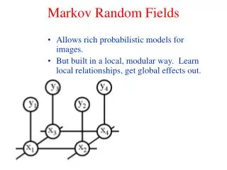
13. Digression: Graph Theory • Define a graph where • is a finite set of vertices/nodes . Usually one node per pixel • is a set of edges where a typical edge is . • We are only considering undirected graphs • ie. and are the same edge • We are only considering simple graphs (no loops) • ie. Graphs that do not contain edges of the form • Define a Neighbourhood System • and are neighbours if • The neighbourhood of is defined as

14. Examples of Graphs: Neighbourhood Systems 4-connected neighbourhood system 8-connected neighbourhood system

15. Definition: Cliques • A clique in the graph contains either • A single node • A subsets of nodes which are mutual neighbours. • is maximal if no other node can be added to the clique without violating the full connectedness property • is the set of all maximal cliques defined on .

16. Gibbs Random Field • Consider the following prior definition • This is known as a Gibbs Random Field • - is a function associated with a maximal clique and is often called a potential. We design each such that undesirable configurations of result in large potentials • is called the partition function and acts as a normalisation constant.

17. Hammersley-Clifford Theorem • States the equivalence of Gibbs and Markov Random Fields. • So the expression for on the last slide describes the prior for an MRF. • Subject to the positivity condition • The local conditional probabilities can be derived as Any maximal clique of which belongs to

18. Priors for 4 connected neighbourhoods • Because the maximal cliques are single edges we can simply the local conditionality to • A smoothess prior for an “unordered” label field • A smoothness prior for an “ordered” or continuous label field

19. Priors for 4 connected neighbourhoods 0 ? 0 0 Given this particular neighbourhood 1 is more likely for . 1 • 8 connected neighbourhoods are more difficult to write priors for because the cliques all have 4 nodes.

20. Putting it all together • We now have expressions for both the prior and likelihood

21. Putting it all together • The posterior is • is referred to as the energy. • Maximising the Posterior is equivalent to minimising the energy. • But how do we find ?

22. Optimising our Framework • Because of the pairwise interactions in the prior optimisation is difficult. Exhaustive search is intractable. • Popular Methods • Sampling (MCMC) with Simulated Annealing (SA) • Gibbs Sampler (Geman & Geman) • Metropolis-Hastings • Loopy Belief Propagation (Pearl) • Iterated Conditional Modes (Besag) • GraphCut • Max-Flow/Min-Cut (Ford & Fulkerson) • Push-Relabel (Goldberg & Tarjan)

23. Iterated Conditional Modes • Given an initial guess of the label field • Visit all nodes in the graph in some order • For each node chose that maximises the local conditional posterior • If has not been visited yet then use instead of • Iterate until convergence.

24. Example Calculation • Estimates local minimum of overall energy . • Good initial guess required • Use Maximum Likehood Estimate perhaps. 0 ? 0 0 1

25. Scan Orders • Random Order • Visit pixels in a different random order at each iteration • Forward/Backward Raster Scan • Each pixel visited twice in each iteration to avoid propagation bias. • Checkerboard Scan • Update every 3rd pixel along every row and column simultaneously. • Offset by 1 and repeat procedure (9 times for 1 iteration). • Neighbourhoods of every 3rd pixel do not overlap so can be implemented as a concurrent update (ie. hardware)

26. Motion Detection Example • Initial Guess using simple threshold • Define Likelihood Energies • Estimate based on initial segmentation • Define Prior Energy (Pairwise Potential) (4 connected neighbourhood)

27. Motion Detection Example • More details • Checkerboard scan used for efficiency reasons (Matlab slow for large for loops). • 10 iterations maximum but will terminate if no pixels change label after an iteration.

28. “Previous” frame “Current” frame

29. First Iteration Final Iteration

30. Iterations Playback at 1 Iteration per second

31. Iterations

32. Final Iteration Final Iteration

33. Conditional Random Fields • Often we like to adapt the prior to data (data-driven prior) • Eg. Suspend spatial smoothness across edges, makes segmentation boundaries “stick” to edges. • Define new pairwise potential • This is an example of a data-driven prior for the motion detection algorithm

34. MRF Final Iteration Final Iteration