Linear Programming
Learn the basic concepts of Linear Programming models and methods of solving them on a computer. Overview of LP's role in solving planning problems and its application in industries like Economics, Engineering, Mathematics, Agriculture, Business, Transport, and Manufacturing.

Linear Programming
E N D
Presentation Transcript
Linear Programming Transportation Networks CIVE 744
Objective • Understand the basic concepts of Linear Programming models and learn basic methods of solving them on computer.
Index • I. Introduction (brief summary) a. Overview b. Structure of a linear programming model (objective function, variables and constraints). • II. Solution of a Linear Programming Problem a. Verbal Description of a problem and symbolic formulation b. Graphical solution • III. Computer solving of a LP model a. Excel solving solution b. Lindo solving solution
I. Introduction • OVERVIEW • Linear programming (LP) can ease the task of solving a particular type of planning problem. LP is a mathematical method or set of procedures to solve and interpret the results of a model of Linear functions that in conjunction represents a phenomenon, generally related to production or industry environments. • The mathematical technique for solving LP problems was developed by George Dantzig in 1947 to solve planning problems in the U.S. Air Force. • Practical applications of LP: • Economicss • Engineering • Mathematics • Agriculture • Business • Transport • Manufacturing
I. Introduction • Structure of a LP Model • To analyse a problem using LP, it must be moulded into a particular structure that at least must contain the following components: • Objective – to obtain the best or optimal solution • Activities or decision variables – What to do? • Constraints or restrictions – Limits on the availability of a resource
II. Solution of a LP problemVerbal description Two Mines Company The Two Mines Company own two different facilities that produce an ore which, after being crushed, is graded into three classes: high, medium and low-grade. The company has contracted to provide a smelting plant with 12 tons of high-grade, 8 tons of medium-grade and 24 tons of low-grade ore per week. The two mines have different operating characteristics as detailed below. Mine Cost per day ($) Production (tons/day) High Medium Low X 180 6 3 4 Y 160 1 1 6 How many days per week should each mine be operated to fulfill the smelting plant contract?
II. Solution of a LP problemSymbolic Formulation Variables These represent the "decisions that have to be made" or the "unknowns". x = number of days per week mine X is operated y = number of days per week mine Y is operated Note here that x >= 0 and y >= 0. Constraints Ore production constraints - balance the amount produced with the quantity required under the smelting plant contract OreHigh 6x + y >= 12 Medium 3x + y >= 8 Low 4x + 6y >= 24 Days per week constraint - we cannot work more than a certain maximum number of days a week e.g. for a 5 day week we have x <= 5 y <= 5
II. Solution of a LP problemSymbolic Formulation Objective Again in words our objective is to minimize cost which is given by Z = 180x + 160y Hence we have the complete mathematical representation of the problem as: Minimize Z= 180x + 160y Subject to 6x + y >= 12 3x + y >= 8 4x + 6y >= 24 x <= 5 y <= 5 x,y >= 0
II. Solution of a LP problemSymbolic Formulation Optimal Solution X= 1.71 Y= 2.86 Z = 765.71

