Download

1 / 25
250 likes | 462 Views
Mismatching Perturbations at the Lateral Boundaries in Limited-Area Ensemble Forecasting. … or why limited-area ensemble forecasting can be more difficult than global ensemble forecasting. Jean-François Caron . Pros. Cons. Simple. No small-scales in the ensemble mean.

E N D
Mismatching Perturbations at the Lateral Boundaries in Limited-Area Ensemble Forecasting … or why limited-area ensemble forecasting can be more difficult than global ensemble forecasting Jean-François Caron
Pros Cons Simple No small-scales in the ensemble mean Ensemble Coherence: No mismatch between the IC from the two ensembles No small-scales in the IC perturbations Not appropriate for short-term forecasting & Perturbations Downscaling Small-scales in the ensemble mean No small-scales in the IC perturbations interpolation Perturbation Coherence: No mismatch between the ensemble perturbations IC perturbations derived from LAM Forecasts Small-scales in the ensemble mean Complex & Small-scales in the ensemble perturbations Ensemble method Risk of generating mismatches in the ensemble perturbations at the LBCs Appropriate for short-term forecasting and for ensemble DA From interpolation Limited-Area EPS: 3 approaches & FullFields Downscaling interpolation
Outline • Description of a 1.5 km ETKF-based limited-area EPS for research purposes • An example of spurious perturbations triggered by mismatches between IC and LBC perturbations • To alleviate mismatches: A perturbation blending approach called ‘the scale-selective ETKF’ Impact of the new method on • Forecast performance • Ensemble-derived background error covariances
Introduction • MOGREPS-G (60 km) – operational • MOGREPS-R (18 km) - operational • ETKF-1.5 km - research Purpose of this convective-permitting EPS • Examine 1-h forecast error covariances for the benefit of a NWP-based nowcasting system in development (Bannister et al., 2011,Tellus) • Predictability studies of very short-term weather events (Migliorini et al., 2011, Tellus) • Test hybrid VAR DA at convective scale 432 km 540 km
ETKF 1.5km: The setup • Control analysis from 3DVAR SUK 1.5km 1-h cycle with cloud and latent heat nudging and UK 4km LBC • 23 IC perturbations are produced by the ETKF using +1h forecast perturbations and the locations and the estimated errors of the assimilated observations. • Surface obs, Aircrafts • Radio-sondes • GPS, radiances • No localizations • Variable multiplicative inflation factor derived from surface obs (u, v, T) and aircraft data (u ,v, T) • No representation of model errors • LBC taken from MOGREPS-R
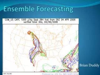
ETKF 1.5km - Case study #3 00Z 05/12/2009 21Z 04/12/2009 00Z 05/12/2009 03Z 05/12/2009
Relative difference (%) -20% +53% -50 -60 -25 -30 0 0 25 25 60 50 % Domain average =+9.9% Comparison of psurf spread MOGREPS-R : 12h fcst ETKF 1.5km : 1-h fcst hPa fields valid at 06z 05/12/2009
Overestimation of psurf spread The Horror Movie The time-evolution of surface pressure perturbation in ensemble member #8 + 1 min + 5 min + 15 min + 30 min + 60 min + 90 min hPa
CTRL LBC 1-h Incremental LBC Update (ILBCU) Sources of discontinuities at the LB (1) • The Incremental Analysis Update (IAU, i.e., how we add the IC perturbations) Initial Conditions Lateral Boundary Conditions Pert. Xa Pert. LBC Pert. LBC Xa CTRL Xa t t+30m t t+30m t-30m t-30m 1-h IAU
Sources of discontinuities at the LB (1) • Relative difference in psurf spread : 1.5km ETKF vs. MOGREPS-R IAU only IAU + ILBCU Other sources of discontinuities between IC and the LBC must be present -20% +41% +53% -50 -60 -25 -30 0 0 25 25 60 50 -50 -60 -25 -30 0 0 25 25 60 50 % % Domain average =+9.90% Domain average =+9.95% 1h forecast valid at 06z 05/12/2009
Perturbations Downscaling • Relative difference in psurf spread : 1.5km ETKF vs. MOGREPS-R Perturbation Downscaling ETKF with ILBCU +41% -50 -60 -25 -30 0 0 25 25 60 50 -50 -60 -25 -30 0 0 25 25 60 50 % % Domain average =+9.95% Domain average =-0.15% 1h forecast valid at 06z 05/12/2009
Sources of discontinuities at the LB (2) • The construction of the IC perturbations Comparison of the ensemble perturbations from MOGREPS-R and the 1.5km-ETKF (at low resolution)
Sources of discontinuities at the LB (2) • The construction of the IC perturbations Comparison of the ensemble perturbations from MOGREPS-R and the 1.5km-ETKF (at low resolution)
Large-scale IC perturbations Low-Pass Filtering step Full IC perturbations High-Pass Filtering step ETKF step 1h small-scale forecast perturbations ETKF small-scale IC perturbations The Scale-Selective ETKF (SSETKF) Large-scale perturbation downscaling Driving-EPS forecast perturbations on LAM domain LAM 1h forecast perturbations Small-scale IC perturbations derived from LAM Forecasts
Three flavours of SSETKF SSETKF-F48-96 SSETKF-F96-192 SSETKF-F192-384
SSETKF: Impact on psurf spread • Relative difference in psurf spread : 1.5km ETKF vs. MOGREPS-R Perturbation Downscaling ETKF-ILBCU SSETKF-F48-96 SSETKF-F96-192 SSETKF-F192-384 -50 -60 -25 -30 0 0 25 25 60 50 %
SSETKF: Impact on precipitation • Verification of 1-h precipitation rate (Brier Score) relative to the ETKF Positive (Negative) means a better (worse) forecasts than the ETKF
SSETKF: Impact on B 1 Global and LAM Parameter transform 2 • The Met Office VAR control variable transform auto covariances only Vertical transform 3 Horizontal transform LAM 4 Global
SSETKF: Impact on B • Degree of linear balance between mass and rotational wind Degree of balance
SSETKF: Impact on B • Horizontal correlation lenghtscales based on a SOAR function
SSETKF: Impact on B • Vertical auto-correlations with model level 30 (~700 hPa)
Summary and discussion • As expected, applying the ETKF approach in a limited-area EPS generates mismatches between IC and LBC perturbations • This is likely to be true for all current limited-area EnDA approach • In our small domain, discontinuities were found to introduce significant spurious perturbations in the pressure field. • This is likely to be less important in larger domains. • Results from the scale-selective ETKF showed that mismatches at low wave numbers were responsible for the spurious perturbations. • The scale-selective ETKF has also improved slightly some other variables compared to both the ETKF and perturbation downscaling. • In terms of background error covariances, perturbation mismatches at the LBCs tend to: • Significantly reduce the degree of balance between mass and rotational wind • Reduce horizontal and vertical correlation lengths
Summary and discussion Pros and Cons of the scale-selective (or blending) approach • Ensures that an a priory specified component of the IC perturbations is coherent with the driving EPS • The small scale IC perturbations are constructed without the knowledge of the large scale perturbations • The small scale IC perturbations could potentially be incoherent with the large scale component. Scale-selection is potentially better than traditional methods but is not the optimal approach. What’s the optimal approach?