Download

1 / 12
120 likes | 509 Views
Levering and Unlevering the Cost of Equity. Unlevered Cost of Equity.

E N D
Unlevered Cost of Equity • Franco Modigliani and Merton Miller postulated that the market value of a company’s economic assets, such as operating assets (Vu) and tax shields (Vtax) should equal the market value of its financial claims, such as debt (D) and equity (E) • Vu + Vtxa =Enterprise Value = D + E
Unlevered Cost of Equity (Contd.) • A second result of Modigliani and Miller’s work is that the total risk of the company’s economic assets, operating and financial, must equal the total risk of the financial claims against those assets: • [(Vu)/(Vu +Vtxa)]×(ku)] + [(Vtxa)/(Vu +Vtxa)]×(ktxa)] =[(D)/(D +E)]×(kd)] + [(E)/(D+E)]×(ke)] • Ku = Unlevered cost of equity • Ktxa = Cost of capital for the company’s interest tax shields • Kd = Cost of debt • Ke = Cost of equity
Unlevered Cost of Equity (Contd.) • ku and ktxa are unobservable • We must therefore impose additional restrictions to solve for ku. • If debt is a constant proportion of enterprise value (i.e., debt grows as the business grows), ktxa should be equal to ku. • Imposing this restriction leads to: • [(Vu)/(Vu +Vtxa)]×(ku)] + [(Vtxa)/(Vu +Vtxa)]×(ku)] =[(D)/(D +E)]×(kd)] + [(E)/(D+E)]×(ke)] • Ku =[(D)/(D +E)]×(kd)] + [(E)/(D+E)]×(ke)]
Unlevered Cost of Equity When ktxa Equals kd • Some financial analysts model the required return on interest tax shields equal to the cost of debt. In this case: • [(Vu)/(Vu +Vtxa)]×(ku)] + [(Vtxa)/(Vu +Vtxa)]×(kd)] =[(D)/(D +E)]×(kd)] + [(E)/(D+E)]×(ke)] • Multiplying both sides by enterprise value: • Vuku +Vtxakd = Dkd + Eke • Vuku = (D-Vtxa)kd + Eke • ku = [(D-Vtxa)/(D-Vtxa+E)] kd + [(E )/(D-Vtxa+E)] ke
Unlevered Cost of Equity When Rupee Level of Debt • If ktxa = ku • ku =[(D)/(D +E)]×(kd)] + [(E)/(D+E)]×(ke)] • If ktxa = kd • ku = [(D×(1-Tm)/(D×(1-Tm) +E)]×(kd)] + [(E)/(D×(1-Tm )+E)]×(ke)] • Tm =Marginal tax rate • The above result is obtained by substituting: Vtxa = (D ×kd ×Tm)/kd = D ×Tm
The Levered Cost of Equity: Rupee Level of Debt Fluctuates • ktxa = ku • ke = ku +(D/E)×(ku – kd) • ktxa= kd • ke = ku +[(D-Vtxa)/E)]×(ku – kd)
The Levered Cost of Equity: Rupee Level of Debt is Constant • ktxa = ku • ke = ku +(D/E)×(ku – kd) • ktxa= kd • ke = ku +(1-Tm)(D/E)×(ku – kd)
The Levered Beta: Rupee Level of Debt Fluctuates • ßtxa = ßu • ße = ßu +(D/E)×(ßu – ßd) • ßtxa= ßd • ße = ßu +[(D-Vtxa)/E)]×(ßu – ßd)
The Levered Beta: Rupee Level of Debt is Constant • ßtxa = ßu • ße = ßu +(D/E)×(ßu – ßd) • ßtxa= ßd • ße = ßu +(1-Tm)(D/E)×(ßu – ßd)
The Levered Beta: Rupee Level of Debt is Constant, Debt Risk-Free • ßtxa = ßu • ße = (1+D/E)×ßu • ßtxa= ßd • ße = ßu +[1+(1-Tm)(D/E)]×ßu