Structure alignment
Structure alignment. Or, What is a correspondence set anyway?!. Topic 12. Chapter 16, Du and Bourne “Structural Bioinformatics”. Alignment vs. superposition. Structural alignment attempts to establish homology between two or more polymer structures based on their shape and 3D structure.


Structure alignment
E N D
Presentation Transcript
Structure alignment Or, What is a correspondence set anyway?! Topic 12 Chapter 16, Du and Bourne “Structural Bioinformatics”
Alignment vs. superposition • Structural alignment attempts to establish homology between two or more polymer structures based on their shape and 3D structure. • Structural alignment requires no a priori knowledge of equivalent positions. • Structural alignment is a valuable tool for the comparison of proteins with low sequence similarity, where evolutionary relationships between proteins cannot be easily detected by standard sequence alignment techniques. • Conversely, simple structural superpositionuses knowledge of at least some equivalent residues to guide a rigid body superposition. • The most basic possible comparison between protein structures makes no attempt to align the input structures. • Requires a precalculated alignment as input to determine which of the residues in the sequence are intended to be considered in the RMSD calculation.
Structure alignment Structure alignments are based on structuresimilarity, from which sequence alignments can be trivially extracted. Due to computational complexity, most structural alignments are pairwise, but multiple alignment methods do exist. + First step Second step
Dynamic programming and sequence alignment To really understand structure alignment, you need to understand sequence alignment... • Dynamic programming (DP) is an algorithm originally developed by Richard Bellman in the early 1950s for “multistage decision processes.” DP methods solve optimization problems, very useful in bioinformatics applications, for example sequence alignment. Even though there are a large number of possible solutions, but only one (or a few) best solution(s). • Foundation: Any partial sub-path ending at a point along the true optimal path must itself be an optimal path leading up to that point. So the optimal path can be found by incremental extensions of optimal sub-paths, leading to a recursive algorithm that is (typically) guaranteed to produce the best answer. • There are two major types of optimal DP sequence alignments: Global(Needleman-Wunsch) and local(Smith-Waterman) alignments. • Based on the assumption of independence, where the score of a residue (mis)match is unaffected by other pairs, thus joint probability! For example… ASCTVL ATCAVI Based on the magic of logarithms
Substitution (scoring) matrix Substitution matrices are composed of log-ratios that compare observed pairs to background expectation. S(ij) > 0 indicate ‘preferred’ matches. For example, the BLOSUM-62 matrix…
Dynamic Programming (DP) Match: +5 Mismatch: -2 Insertion/deletion: -6 Sean Eddy, 2004, Nature Biotechnology
Back to structure alignment Independence is not a valid assumption in structure because… Similarly, in RNA… For example… That is, the probability of mutating the above lysine to X, p(KX), is NOT independent of the aspartate. This is, of course, the reality in sequence alignment too, but we ignore this fact because we are treating the protein as a 1D sequence that doesn’t reveal those details.
Rigid body treatment ≠ independence of positions Structure alignment treats proteins as rigid bodies, leading to an even more serious violation of independence. Rotation of purple by 90o also rotates the green That is, adjusting the position of the purple residue, for example, to maximize overlap with its target will also alter the position of the green residue because they rigidly related.
Formalizing the structure alignment problem Given two sets of points A = (a1, a2, …, an) and B = (b1,b2,…bm) in Cartesian space, find the optimalsubsets A(P)and B(Q) with |A(P)| = |B(Q)|, and find the optimalrigid body transformation Gbetween the two subsets A(P) and B(Q) that minimizes a given distance metric D over all possible rigid body transformation G, i.e. The two subsets A(P) and B(Q) define a “correspondence”, and p = |A(P)| = |B(Q)|is called the correspondence length. Naturally, the correspondence length is maximal when A(P) and B(Q) are similar. Therefore there are essentially two problems in structure alignment: (i.) Find the correspondence set (which is NP-hard), and (ii.) Find the alignment transform (which is O(n)).
Just to clarify… In the structure alignment literature, you will frequently encounter coordinate root mean squared deviation, which is just like RMSD except B describes a coordinate transformation of b. Where B describes a coordinate transformation of b.
Common structure alignment methods • DALI: Uses 2D distance matrices between CA atomsto represent each structure. Conceptually, the alignment problem is then straightforward, you must simply maximally overlay the matrices (as described in an earlier cartoon). • Holm and Sander. Protein structure comparison by alignment of distance matrices. J Mol Biol 1993, 233:123-128. • CE (Combinatorial extension): Uses characteristics of local geometry to seed structural alignments and then joins these regions of local similarity (called aligned fragment pairs, AFPs) into an “optimal” path for the full alignment. Bottom-up approach. • Shindyalov and Bourne, Protein structure alignment by incremental combinatorial extension (CE) of optimal path. Prot Eng, 1998, 11:739-747. • SSAP (Sequential Structure Alignment Program ): Uses a “double-dynamic programming” algorithm: high level and low level matrices. Used in CATH classification. • Taylor WR, Orengo CA. 1989b. Protein structure alignment. J Mol Biol 208:l-22 • VAST (Vector AlignmentSearchTool), TM-align and many more……
Overview of the Dali Algorithm Starting with a contact map… Dali attempts to maximize the overlap of the contact maps; however, doing so globally is NP-hard, so the methods focus on local comparisons. Image from Amy Keating at MIT Image from Mark Maciejewski at UConn
Overview of the Dali Algorithm The DALI (Distance matrix alignment) algorithm is based on the matrix comparison methods that we have already introduced. Similarity score: • i and j are equivalent residues in A and B • L is the number of such pairs or the size of the substructure • is the similarity measure based on the CA distance • and iA iB jA jB Structure A Structure B Images and content modified from Mark Maciejewski at UConn
The Dali Algorithm (step by step) Compute distance matrices for both protein A and B Extract a full set of overlapped hexapeptide (6x6) sub-matrices (also called contact patterns) from each matrix Each 6x6 distance matrix from protein A is compared with the 6x6 distance matrix in protein B. (Really?) 6x6 CA distance matrices For example: 6.2 – 12.7 = -6.5
The Dali Algorithm (step by step) Step 1: For each hexapeptide, a distance matrix compares it to every other hexapeptide within its structure. Step 2:Every distance matrix created in step 1 for each protein are compared to each other. “Houston, … we have a problem!” Consider protein A with 100residues, meaning we have 100 - 5 = 95hexapeptides. (95^2)/2 = 4,512contact pattern matrices Consider protein B with 150residues, meaning 150-5 = 145hexapeptides. (145^2)/2 = 10,512contact pattern matrices Even for these two relatively small proteins, there would be 4,512x 10,512= 47,430,144 comparisons between A and B.
The Dali Algorithm (step by step) Each contact pattern in protein A is paired with its most similar pattern in protein B, a process that generates a pair list The list is sorted based on the strength of pair similarity of contact patterns Note that unmatched residues do not contribute to the overall similarity score S. Image from Amy Keating at MIT A note about the similarity measure :We want to maximize the number of equivalent residues while minimize structural variations – it is a tradeoff. That is, if the criteria are so tough that minor structure deviations are not allowed, then the number of matching contact patterns is likely to be very small.
The Dali Algorithm (step by step) Q: How do you calculate f(i,j)? Method 1: Rigid residue-pair similarity score: -- 1.5 Å is the zero level of similarity. -- The only thing that matters is absolute difference, meaning that the same difference at large distances is penalized the same as short distances. Method 2: Elastic similarity score (default): -- Larger differences are tolerate for longer-range contact pairs.
The Dali Algorithm (step by step) 6. Merging contact patterns to form chains and reduce complexity The search space is reduced because only the central contact pattern is retained (actually, the one that gives the smallest average intra-pattern distance).
The Dali Algorithm (step by step) 7.) After removing the overlapping patterns, we are still left with way too many contact patterns to exhaustively compare all possible pairs. Start comparing pairs at random: -- Keep list of positive scores (discard negative scores) -- Keep comparing till your list has 80,000 positive scores Sort the list and keep the best 40,000 contact pattern matches. 8.) End game: Need to find optimal alignment of the 40,000 contact patterns such that the alignment occurs over as wide a range of the structural pair as possible. Using Markov Chain Monte Carlo (MCMC), start with a random contact pattern from the list of 40,000, and then “walk” to another overlapping pattern (must extend the contact pattern by 4 residues) using the standard Metropoliscriterion.
Metropolis Monte Carlo Optimization In Dali… The net result is that scores that improve are always kept, whereas scores that get worse are excepted with some probability.
Statistical significance of Dali alignments Dali uses Z-scoreto show the significance of the alignment A common and practical approach to the problem of assessing alignment significance is to determine if the alignment score is better than one could expect by chance. Dali compares each alignment score against an All-to-All protein structure comparison (normalized by length), which defines the z-score. -- Dali Z-scores > 2 are thought to be meaningful.
Combinatorial Extension (a cursory look) • Similar to Dali in that it also breaks the structure down into a series of small fragments, from which it attempts to reassemble into a complete alignment. • For a pair of proteins A and B, an alignment fragment pair (AFP) is defined as a continuous segment of A aligned against a continuous segment of B of the same size (without gaps). • If n1 and n2 are the lengths of A and B, and AFP length is set to m, then there is a total of possible (n1 m)(n2 m) AFPs. • Only AFPs that meet a given criteria for local similarity are included in the matrix as means of restricting the search space. • An alignment path is calculated as the optimal path through the similarity matrix by linearly progressing through the sequences and extending the alignment with the next possible high-scoring AFP pair.
Combinatorial Extension (a cursory look) • Goal: Find a “good” local alignment for structures of proteins A and B. • Select some initial AFP. • Build an alignment path by incrementally adding AFPs in a way that satisfies the conditions(i.e., stitch AFPs together). • Repeat step (2) until the length of each protein is traversed, or until no “good” AFPs remain. • Optimize the alignment via dynamic programming. • Measure statistical significance. • Questions: • How do we choose the starting AFP? • What are the criteria for adding AFPs to our alignment path? • What does the distance function look like. • When to stop? Or at what point do we know that there no “good” AFPs left?
Combinatorial Extension (a cursory look) • To assess how good the alignment produced by CE is, we can compare it to the alignment of a random pair of structures, and compute the Z-score based on the RMSD distance and number of gaps in the final alignment. • Since CE does not penalize gaps, we can perform additional optimization after the CE is completed in order to remove excess gaps using dynamic programming. • The CE method is highly configurable, which is at once its strength and weakness. Adjusting multiple parameters, such as AFP length m, cutoff distances D0 and D1, and definitions for AFP distances, can result varying alignments and execution speeds. • In general, CE does not outperform previously existing structural alignment methods, such as Dali and VAST: it does better for some pairs of structures, and worse for others.
VAST (a cursory look) VAST = Vector Alignment Search Tool
VAST (a cursory look) 1.) Parse protein structures into SSEs (helices and strands). 2.) Fit vectors to SSEs. 3.) To compare a pair of proteins attempt to superpose as many vectors as possible, subject to constraints. 4.) Evaluate the vector alignment for statistical significance (compute an E-value). 5.) If the vector alignment is significant then proceed to a more detailed residue-to-residue alignment (“refined alignment”). Modified from Tom Madej at GWU
+ VAST in pictures… Modified from Tom Madej at GWU
Double Dynamic Programming (a cursory look) • Use two levels of dynamic programming, a high level scoring matrix and a low level matrix for each high level matrix element. • For each Fijin the high level scoring matrix, it shows how likely it is that the pair is on an optimal alignment. • For each Fij , the likelihood is found by a (low level) optimal alignment with the constraint that Fij is part of the alignment. • The scores along the low level alignments are accumulated in the high level scoring matrix.
DDP cont. • Begin by constructing a series of inter-residue distance vectors between each residue and its nearest non-contiguous neighbors on each protein. • A series of matrices are then constructed containing the vector differences between neighbors for each pair of residues for which vectors were constructed. • Dynamic programming applied to each resulting matrix determines a series of optimal local alignments which are then summed into a "summary" matrix to which dynamic programming is applied again to determine the overall structural similarity.
Stated in a slightly different manner • First level: • Represent each residue by neighborhood vector for C • Compare n versus m neighborhood vectors • Generate optimal alignment based on vector differences and dynamic programming • Second Level: • Add matrix scores if paths cross in a cumulative matrix • Generate optimal alignment based on the cumulative matrix
SSAP = Sequential Structure Alignment Program • Generally, SSAP scores above 80 are associated with highly similar structures. Scores between 70 and 80 indicate a similar fold with minor variations. Structures yielding a score between 60 and 70 do not generally contain the same fold, but usually belong to the same protein class with common structural motifs. • SSAP originally produced only pairwise alignments but has since been extended to multiple alignments as well. • It has been applied in an all-to-all fashion to produce CATH.
Multiple Structure Alignment • Most multiple structure alignments are based on a pile-up combination of pairwise results; however, few algorithms do an All-to-All optimization. • One example of a multiple alignment is Combinatorial Extension Monte Carlo (CE-MC), which is based on a progressive CE multiple alignment strategy, followed by an iterative Metropolis MC refinement.