Download

1 / 36
360 likes | 427 Views
Theory of Turbine Cascades. P M V Subbarao Professor Mechanical Engineering Department. Its Group Performance, What Matters.……. Professor Hermann Schlichting. H. Schlichting’s Approach.

E N D
Theory of Turbine Cascades P M V Subbarao Professor Mechanical Engineering Department Its Group Performance, What Matters.……
H. Schlichting’s Approach • The main incentive of cascade flow investigations is that real progress in the flow problems of turbines will be achieved only by a deeper knowledge of complex flow phenomena. • This requires extensive theoretical calculations which, however, need careful correlation with experiments.
CASCADE FLOW PROBLEMS :H. Schlichting • The very complex cascade flow problem has been split up as follows:- • Two-dimensional flow through cascades. • (a) Incompressible and inviscid flow. • (b) Incompressible, viscous flow. • (c) Compressible flow. • Three-dimensional flow through cascades. • (a) Secondary flow effects at blade root and blade tip. • (b) Effects due to radial divergence of the blades in cascades of rotational symmetry.
Potential flow Analysis of cascades • There are many methods available for potential flow analysis of Cascades • A simple method that works for any infinite linear cascade composed of arbitrary shaped blades separated by a uniform spacing h is called asSingle conformal Transformation method. • This method solves the problem, irrespective of the blade shape, spacing or stagger.
The linear Cascade of Infinite number of blades This physical plane that contains this geometry is called as the Z1plane.
Conformal transformation • For the single conformal transformation, the mapping function is: • where h is the spacing between blades in the linear-cascade in the physical Z1-plane. • Once this transformation is applied, all the blades in the linear cascade system shown in the Z1-plane are transformed into a single contour in the Z2-plane.
Infinite number of Blades in Z2 -- Plane The far upstream and downstream velocities are represented in this plane by : the point source/sink of strength Q & the point vortices (upstream, downstream) at the locations indicated by the filled in circles.
The Capacity of Cascade • The point source of strength Q = V1h cos(α1) represents the flow rate between two blades that is dependent on the horizontal velocity component (V1 cos α1). • The vertical velocity component (V1 sin α1) is represented by a point vortex. • upstream= V1h sin(α1), where V1and α1are the inlet velocity and angle of inclination far upstream of the cascade. • Similarly, the exit conditions (at −∞) in the Z1-plane can be represented by a combination of a sink (−Q) and a vortex (downstream) located at (−1, 0) in the Z2-plane. • The mass conservation in the Z1-plane requires the sink magnitude to be the same as that of the source, while the downstream vertical velocity component, represented by the point vortex (downstream) in the Z2-plane, will change from the upstream value.
The Method The potential flow around the single closed contour in the Z2-plane in the presence of the source (Q) and vortex (upstream) at (+1, 0) and the sink (−Q) and the unknown vortex (downstream) at (−1, 0) is solved using the vortex panel method.
Vortex Panel Method for Design of Cascade Discretize the transformed single contour in to m vortex panels with m + 1 nodes. The vorticity distribution along each panel is linear as shown in the inset.
Method of Solution • In this panel method, the number of unknowns in the form of nodal vorticity strengths is equal to one more than the number of panels (m). • In this problem, the vorticity at the sink location (downstream) is an additional unknown. • Therefore, there are (m+2) unknowns and the same number of equations are required to solve for the unknowns. • The impermeability condition at the control points on the panels and the Kutta condition at the trailing edge yield (m+1) equations. • The extra (m + 2)th equation is given by the fact that in the z1-plane, the change in vertical velocity from far upstream to far downstream of the cascade should be equal to the circulation around one blade.
The Cause Created by a Cascade stagger (β) = 37·5◦, solidity (σ ) = 1·01 and α1 = 53·5◦.
Non-Dimensional Variables for Real Cascade Analysis • Non dimensional deflection: • Loss Coefficient: • Solidity ratio: • Reynolds Number:
Non-Dimensional Design Variables for A Stage • Pressure Coefficient: • Flow Coefficient:
COMPRESSIBLE CASCADE FLOW • This is regarded as very important for basic research on cascades, because the aerodynamic coefficients in most cases depend considerably on both the Mach number and the Reynolds number of the blade. • The independent variation of Mach number and Reynolds number is achieved by installing the cascade wind tunnel in a tank which can be evacuated from 1 atm down to 0.1 atm. • The Mach number range is from M = 0.2 to about 1.1. • The blade length L = 300 mm and the blade chord c = 60 mm. • For one year an extensive programme of pressure distribution measurements has been carried out on cascade blades at high subsonic speeds.
Remarks on Turbine Performance Predictions • TURBINPEER FORMANCE can only be satisfactorily determined by tests on full scale machines. • Such tests, however, reflect the aggregate effect of a large number of features influencing total losses. • For a basic understanding of turbine performance it is necessary to analyze the behavior of individual features. • Development and testing of linear cascades is essential in understanding the losses generated by individual features.
The difference - 1 • A linear cascade differs from blading in a real turbine in two ways. • First, differences occur when the cascade tests are carried out: (1) with a different working fluid; (2) with a different Reynolds number; (3) with a different scale of blade; (4) with a different surface roughness; (5) with a different Mach number. • Differences of this sort, if they occur, are capable of being corrected, with the major proviso that the information is available as to how the correction should be made.
The difference - 2 • Second difference is more fundamental and exist as: • Cascade flow: Uniform inlet conditions & Linear flow. • Turbine flow: Inlet flow containing wakes, disturbances due to preceding flows & Annular flow. • Cascade flow: Walls stationary relative to blades. • Turbine flow: Walls may be moving relative to blades. • Differences of this type are an inherent limitation in the use of stationary linear cascade data. • It is very essential to compare the results of carefully interpreted cascade data with actual turbine performance, • and to deduce from the overall result the magnitude and importance of the errors involved
Cascades, Stage & Turbine • Cascades are classified into: • Stationary cascades : Nozzle Cascades • Moving cascades : Rotor Cascades. • A stage is a combination of a nozzle cascade and rotor cascade with a minimum gap between them. • Number of such Stages together make a turbine