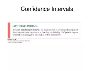
Confidence Intervals
Learn how to compute precise confidence intervals for population estimation using point estimates and standard deviations. Understand the importance of Central Limit Theorem in obtaining accurate estimates. Explore examples and methods for constructing confidence intervals at different confidence levels.

Confidence Intervals
E N D
Presentation Transcript
Confidence Intervals Berlin Chen Department of Computer Science & Information Engineering National Taiwan Normal University Reference: 1. W. Navidi. Statistics for Engineering and Scientists. Chapter 5 & Teaching Material
Introduction • We have discussed point estimates: • as an estimate of a success probability, • as an estimate of population mean, • These point estimates are almost never exactly equal to the true values they are estimating • In order for the point estimate to be useful, it is necessary to describe just how far off from the true value it is likely to be • Remember that one way to estimate how far our estimate is from the true value is to report an estimate of the standard deviation, or uncertainty, in the point estimate • In this chapter, we can obtain more information about the estimation precision by computing a confidence interval when the estimate is normally distributed (Bernoulli trials)
Revisit: The Central Limit Theorem • The Central Limit Theorem • Let X1,…,Xn be a random sample from a population with mean and variance 2 (n is large enough) • Let be the sample mean • Let be the sum of the sample observations. Then if n is sufficiently large, • And approximately sample mean is approximately normal !
Example • Assume that a large number of independent unbiased measurements, all using the same procedure, are made on the diameter of a piston. The sample mean of the measurements is 14.0 cm (coming from a normal population due to the Central Limit Theorem ), and the uncertainty in this quantity, which is the standard deviation of the sample mean , is 0.1 cm • So, we have a high level of confidence that the true diameter is in the interval (13.7, 14.3). This is because it is highly unlikely that the sample mean will differ from the true diameter by more than three standard deviations
Large-Sample Confidence Interval for a Population Mean • Recall the previous example: Since the population mean will not be exactly equal to the sample mean of 14, it is best to construct a confidence interval around 14 that is likely to cover the population mean • We can then quantify our level of confidence that the population mean is actually covered by the interval • To see how to construct a confidence interval, let represent the unknown population mean and let 2 be the unknown population variance. Let X1,…,X100 be the 100 diameters of the pistons. The observed value of is the mean of a large sample, and the Central Limit Theorem specifies that it comes from a normal distribution with mean and whose standard deviation is
Illustration of Capturing True Mean • Here is a normal curve, which represents the distribution of . The middle 95% of the curve, extending a distance of 1.96 on either side of the population mean , is indicated. The following illustrates what happens if lies within the middle 95% of the distribution: 95% of the samples that could have been drawn fall into this category 95% confidence interval
Illustration of Not Capturing True Mean • If the sample mean lies outside the middle 95% of the curve: Only 5% of all the samples that could have been drawn fall into this category. For those more unusual samples the 95% confidence interval fails to cover the true population mean 95% confidence interval
The 95% confidence interval (CI) is So, a 95% CI for the mean is 14 1.96 (0.1). We can use the sample standard deviation as an estimate for the population standard deviation, since the sample size is large We can say that we are 95% confident, or confident at the 95% level, that the population mean diameter for pistons lies, between 13.804 and 14.196 Warning: The methods described here require that the data be a random sample from a population. When used for other samples, the results may not be meaningful Computing a 95% Confidence Interval
Question? • Does this 95% confidence interval actually cover the population mean ? • It depends on whether this particular sample happened to be one whose mean (i.e. sample mean) came from the middle 95% of the distribution or whether it was a sample whose mean (i.e. sample mean) was unusually large or small, in the outer 5% of the population • There is no way to know for sure into which category this particular sample falls • In the long run, if we repeated these confidence intervals over and over, then 95% of the samples will have means (i.e. sample mean) in the middle 95% of the population. Then 95% of the confidence intervals will cover the population mean
Extension • We are not always interested in computing 95% confidence intervals. Sometimes, we would like to have a different level of confidence • We can use this reasoning to compute confidence intervals with various confidence levels • Suppose we are interested in 68% confidence intervals, then we know that the middle 68% of the normal distribution is in an interval that extends 1.0 on either side of the population mean • It follows that an interval of the same length around specifically, will cover the population mean for 68% of the samples that could possibly be drawn • For our example, a 68% CI for the diameter of pistons is 14.0 1.0(0.1), or (13.9, 14.1)
100(1 - )% CI • Let X1,…,Xn be a large (n > 30) random sample from a population with mean and standard deviation , so that is approximately normal. Then a level 100(1 - )% confidence interval for is • is the z-score that cuts off an area of in the right-hand tail • where . When the value of is unknown, it can be replaced with the sample standard deviation s
Particular CI’s • is a 68% interval for • is a 90% interval for • is a 95% interval for • is a 99% interval for • is a 99.7% interval for Note that even for large samples, the distribution of is only approximately normal, rather than exactly normal. Therefore, the levels stated for confidence interval are approximate.
Example (CI Given a Level) • Example 5.1: The sample mean and standard deviation for the fill weights of 100 boxes are = 12.05 and s = 0.1. Find an 85% confidence interval for the mean fill weight of the boxes. Answer: To find an 85% CI, set 1 - = .85, to obtain = 0.15 and /2 = 0.075. We then look in the table for z0.075, the z-score that cuts off 7.5% of the area in the right-hand tail. We find z0.075 = 1.44. We approximate So the 85% CI is 12.05 (1.44)(0.01) or (12.0356, 12.0644).
Another Example (The Level of CI) • Question: There is a sample of 50 micro-drills with an average lifetime (expressed as the number of holes drilled before failure) was 12.68 with a standard deviation of 6.83. Suppose an engineer reported a confidence interval of (11.09, 14.27) but neglected to specify the level. What is the level of this confidence interval? Answer: The confidence interval has the form . We will solve for z/2, and then consult the z table to determine the value of . The upper confidence limit of 14.27 therefore satisfies the equation 14.27 = 12.68 + z/2(6.83/ ). Therefore, z/2 = 1.646. From the z table, we determine that /2, the area to the right of 1.646, is approximately 0.05. The level is 100(1 - )%, or 90%.
More About CI’s (1/2) • The confidence level of an interval measures the reliability of the method used to compute the interval • A level 100(1 - )% confidence interval is one computed by a method that in the long run will succeed in in covering the population mean a proportion 1 - of all the times that it is used • In practice, there is a decision about what level of confidence to use • This decision involves a trade-off, because intervals with greater confidence are less precise
More About CI’s (2/2) 100 samples 68% confidence intervals 95% confidence intervals 99.7% confidence intervals
Probability vs. Confidence • In computing CI, such as the one of diameter of pistons: (13.804, 14.196), it is tempting to say that the probability that lies in this interval is 95% • The term probability refers to random events, which can come out differently when experiments are repeated • 13.804 and 14.196 are fixed not random. The population mean is also fixed. The mean diameter is either in the interval or not • There is no randomness involved • So, we say that we have 95% confidence that the population mean is in this interval
Determining Sample Size • Back to the example of diameter of pistons: We had a CI of (13.804, 14.196). • This interval specifies the mean to within 0.196. Now assume that the interval is too wide to be useful Question: Assume that it is desirable to produce a 95% confidence interval that specifies the mean to within 0.1 • To do this, the sample size must be increased. The width of a CI is specified by . If we know and is specified, then we can find the n needed to get the desired width • For our example, the z/2 = 1.96 and the estimated standard deviation of the population is 1. So, 0.1 =1.96(1)/ , then the n accomplishes this is 385 (always round up)
One-Sided Confidence Intervals (1/2) • We are not always interested in CI’s with an upper and lower bound • For example, we may want a confidence interval on battery life. We are only interested in a lower bound on the battery life. There is not an upper bound on how long a battery can last (confidence interval =(low bound,∞ ) ) • With the same conditions as with the two-sided CI, the level 100(1-)% lower confidence bound for is and the level 100(1-)% upper confidence bound for is
One-Sided Confidence Intervals (2/2) • Example: One-sided Confidence Interval (for Low Bound)
Confidence Intervals for Proportions • The method that we discussed in the last section (Sec. 5.1) was for mean from any population from which a large sample is drawn • When the population has a Bernoulli distribution , this expression takes on a special form (the mean is equal to the success probability) • If we denote the success probability as and the estimatefor as which can be expressed by • A 95% confidence interval (CI) for p is : the sample size :number of sample items that success
Comments • The limits of the confidence interval contain the unknown population proportion • We have to somehow estimate this ( ) • E.g., using • Recent research shows that a slight modification of and an estimate of improve the interval • Define • And
CI for • Let be the number of successes in independent Bernoulli trials with success probability , so that • Then a 100(1 - )% confidence interval for is • If the lower limit is less than 0, replace it with 0. • If the upper limit is greater than 1, replace it with 1
Small Sample CI for a Population Mean • The methods that we have discussed for a population mean previously require that the sample size be large • When the sample size is small, there are no general methods for finding CI’s • If the population is approximately normal, a probability distribution called the Student’s t distribution can be used to compute confidence intervals for a population mean
More on CI’s • What can we do if is the mean of a small sample? • If the sample size is small, s may not be close to , and may not be approximately normal. If we know nothing about the population from which the small sample was drawn, there are no easy methods for computing CI’s • However, if the population is approximately normal, will be approximately normal even when the sample size n is small. It turns out that we can use the quantity , but since s may not be close to , this quantity instead has a Student’s distribution with n-1 degrees of freedom, which we denote
Student’s t Distribution (1/2) • Let X1,…,Xn be a small (n < 30) random sample from a normal population with mean . Then the quantity has a Student’s t distribution with n -1 degrees of freedom (denoted by tn-1). • When n is large, the distribution of the above quantity is very close to normal, so the normal curve can be used, rather than the Student’s t
Student’s t Distribution (2/2) • Plots of probability density function of student’s t curve for various of degrees • The normal curve with mean 0 and variance 1 (z curve) is plotted for comparison • The t curves are more spread out than the normal, but the amount of extra spread out decreases as the number of degrees of freedom increases
More on Student’s t • Table A.3 called a t table, provides probabilities associated with the Student’s t distribution
Examples • Question 1: A random sample of size 10 is to be drawn from a normal distribution with mean 4. The Student’s t statistic is to be computed. What is the probability that t > 1.833? • Answer: This t statistic has 10 – 1 = 9 degrees of freedom. From the t table, P(t > 1.833) = 0.05 • Question 2: Find the value for the distribution whose lower-tail probability is 0.01 • Answer: Look down the column headed with “0.01” to the row corresponding to 14 degrees of freedom. The value for t = 2.624. This value cuts off an area, or probability, of 1% in the upper tail. The value whose lower-tail probability is 1% is -2.624
Student’s t CI • Let X1,…,Xn be a small random sample from a normal population with mean . Then a level 100(1 - )% CI for is • To be able to use the Student’s t distribution for calculation and confidence intervals, you must have a sample that comes from a population that it approximately normal Two-sided CI
Other Student’s t CI’s • Let X1,…,Xn be a small random sample from a normal population with mean • Then a level 100(1 - )% upper confidence bound for i • Then a level 100(1 - )% lower confidence bound for is • Occasionally a small sample may be taken from a normal population whose standard deviation is known. In these cases, we do not use the Student’s t curve, because we are not approximating with s. The CI to use here, is the one using the z table, that we discussed in the first section one-sided CI one-sided CI
Determine the Appropriateness of Using t Distribution (1/2) • We have to decide whether a population is approximately normal before using t distribution to calculate CI • A reasonable way is construct a boxplot or dotplot of the sample • If these plots do not reveal a strong asymmetry or any outliers, the it most cast the Student’s t distribution will be reliable • Example 5.9: Is it appropriate to use t distribution to calculate the CI for a population mean given a a random sample with 15 items shown below 580, 400, 428, 825, 850, 875, 920, 550, 575, 750, 636, 360, 590, 735, 950. Yes !
Determine the Appropriateness of Using t Distribution (2/2) • Example 5.20: Is it appropriate to use t distribution to calculate the CI for a population mean given a a random sample with 11 items shown below 38.43, 38.43, 38.39, 38.83, 38.45, 38.35, 38.43, 38.31, 38.32, 38.38, 38.50. No !
CI for the Difference in Two Means (1/2) • We also can estimate the difference between the means and of two populations and • We can draw two independent random samples, one from and the other one from , each of which respectively has sample means and • Then construct the CI for by determining the distribution of • Recall the probability theorem:Let and be independent, with and Then • And
CI for the Difference in Two Means (2/2) • Let be a large random sample of size from a population with mean and standard deviation , and let be a large random sample of size from a population with mean and standard deviation . If the two samples are independent, then a level 100(1- )% CI for is • When the values of and are unknown, they can be replaced with the sample standard deviations and Two-sided CI
CI for Difference Between Two Proportions (1/3) • Recall that in a Bernoulli population, the mean is equal to the success probability (population proportion) • Let be the number of successes in independent Bernoulli trials with success probability , and let be the number of successes in independent Bernoulli trials with success probability , so that and • The sample proportions following from the central limit theorem ( and are large)
CI for Difference Between Two Proportions (2/3) • The difference satisfies the following inequality for 95% of all possible samples • Traditionally in the above inequality, is replaced by and is replaced by Two-sided CI
CI for Difference Between Two Proportions (3/3) • Adjustment (In implementation): • Define • The 100(1-)% CI for the difference is • If the lower limit of the confidence interval is less than -1, replace it with -1 • If the upper limit of the confidence interval is greater than 1, replace it with 1
Small-Sample CI for Difference Between Two Means (1/2) • Let be a random sample of size from a normal population with mean and standard deviation , and let be a random sample of size from a normal population with mean and standard deviation . Assume that the two samples are independent. If the populations do not necessarily have the same variance, a level 100(1- )% CI for is • The number of degrees of freedom, , is given by (rounded down to the nearest integer) Two-sided CI
Small-Sample CI for Difference Between Two Means (2/2) • If we further know the populations and are known to have nearly the same variance. Then a 100(1-)% CI for is • The quantity is the pooled variance, given by • Don’t assume the population variance are equal just because the sample variance are close Two-sided CI
CI for Paired Data (1/3) • The methods discussed previously for finding CI’s on the basis of two samples have required the samples are independent • However, in some cases, it is better to design an experiment so that each item in one sample is paired with an item in the other • Example: Tread wear of tires made of two different materials
CI for Paired Data (2/3) • Let be sample pairs. Let . Let and represent the population means for and , respectively. We wish to find a CI for the difference . Let represent the population mean of the differences, then . It follows that a CI for will also be a CI for • Now, the sample is a random sample from a population with mean , we can use one-sample methods to find CIs for
CI for Paired Data (3/3) • Let be a small random sample (n < 30) of differences of pairs. If the population of differences is approximately normal, then a level 100(1-)% CI for is • If the sample size is large, a level 100(1-)% CI for is • In practice, is approximated with
Summary • We learned about large and small CI’s for means • We also looked at CI’s for proportions • We discussed large and small CI’s for differences in means • We explored CI’s for differences in proportions

