Download
1 / 66
660 likes | 906 Views
UofO- Geology 619. Electron Beam MicroAnalysis- Theory and Application Electron Probe MicroAnalysis - (EPMA). Imaging: (Analog imaging and X-ray mapping). Modified from Fournelle, 2006). “A picture is worth a thousand words”

E N D
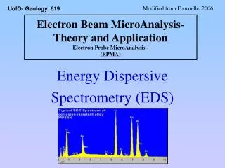
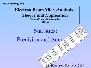
UofO- Geology 619 Electron Beam MicroAnalysis- Theory and ApplicationElectron Probe MicroAnalysis -(EPMA) Imaging: (Analog imaging and X-ray mapping) Modified from Fournelle, 2006)
“A picture is worth a thousand words” The more we know about how images are acquired and processed, the better we can present research results graphically. Additionally, 2 or 3 dimensional information about specimens can be extracted from some images.
Image Acquisition Secondary electron images Backscatter electron images X-ray maps (WDS, EDS) Dot maps Counter (pulse count) maps Cathodo-luminescence images Microscope (camera) images
Image Processing & Analysis Image acquisition Image storage Image defects/correction Image enhancement Segmentation and thresholding Processing in frequency space Processing binary images Image measurements Image presentation
Software • MicroImage (interfaces with SX51) or Probe Image (interfaces with SX100) • Probe for EPMA (SX51/SX100 and JEOL 8900/8200 and 8500) • Matrox Frame grabber (interfaces with SX100 video display) • NIH/Scion Image rsb.info.nih.gov/nih-image/more-docs/Tutorial/Contents.html • Image-Pro and Adobe Photoshop • Books • The Image Processing Handbook by John C. Russ, 3rd Ed, 1999, CRC Press (he teaches a week-long short course at North Carolina State University) • Quick Photoshop for Research, A guide to digital imaging for Photoshop 4xd, 5x,6x,7x by Jerry Sedgewick, 2002, Kluwer Academic/Plenum Publishers Resources:
Optical scanning (Nikon slide scanner) • Use the Nikon slide scanner to scan your entire section for: • 1. Documentation • 2. Identify regions of interest • 3. Use Click and Move feature (image registration)
Secondary electron images Everhart-Thornley detector: low-energy secondary electrons are attracted by +200 V on grid and accelerated onto scintillator by +10 kV bias; light produced by scintillator (phosphor surface) passes along light pipe to external photomultiplier (PM) which converts light to electric signal. Back scattered electrons also detected but less efficiently because they have higher energy and are not significantly deflected by grid potential. (image and text from Reed, 1996, p. 37) SE imaging: the signal is from the top 5 nm in metals, and the top 50 nm in insulators. Thus, fine scale surface features are imaged. The detector is located to one side, so there is a shadow effect – one side is brighter than the opposite.
BSE images A solid-state (semi-conductor) backscattered electron detector (a) is energized by incident high energy electrons (~90% E0), wherein electron-hole pairs are generated and swept to opposite poles by an applied bias voltage. This charge is collected and input into an amplifier (gain of ~1000). (b) It is positioned directly above the specimen, surrounding the opening through the polepiece. In our BSE detector, we can modify the amplifier gain: BSE GMIN or BSE GMAX. BSE imaging: the signal comes from the top ~.1 um surface; solid-state detector is sensitive to light (and red LEDs). Above, 5 phases stand out in a volcanic ash fragment Goldstein et al, 1992, Fig 4.24, p. 184
There are several alternative type SEM images sometimes found in BSE or SE imaging: (left) channeling (BSE) and (right) magnetic contrast (SE). Fournelle has found BSE images of single phase metals with crystalline structure shown by the first effect, and suspect the second effect may be the cause of problems with some Mn-Ni phases. Variations on a theme Crystal lattice shown above, with 2 beam-crystal orientations: (a) non-channeling, and (b) channelling.Less BS electrons get out in B, so darker. From Newbury et al, 1986, Advanced Scanning Electron Microscopy and X-ray Microanalysis, Plenum, p. 88 and 159.
Electron backscatter diffraction is a relatively new and specialized application whereby a specimen (say single crystal) is tilted acutely (~70°) in an SEM with a special detector (‘camera’). The electron beam interacts with the crystal lattice and the lattice planes will diffract the beam, with the backscattered electrons striking the detector, yielding sets of intersecting lines, which then can be indexed and crystallographic data deduced. EBSD* * Also referred to as Kossel X-ray diffraction, and Kikuchi patterns. (Left) EBSD pattern from marcasite (FeS2) crystal. (Right) Diagram showing formation of cone of diffracted electrons formed from a divergent point source within a specimen. Dingley and Baba-Kishi, 1990, Electron backscatter diffraction in the scanning electron microscope, Microscopy and Analysis, May.
BSE and SE Detectors on our SX51/SX100 Annular BSE detectors Plates for +voltage for SE detector View from inside, looking up obliquely (image taken by handheld digital camera)
Cathodo-luminescence This is an optical phenomenon. CL occurs in semiconductors, be they man-made or natural (i.e., some minerals). Electrons in the valence band of these materials are excited into the conduction band for a brief time; subsequently these electrons recombine with the holes left in the valence band. The energy difference is released as a photon of wavelength of light. Two commonly used applications are Locating strain (lattice mismatch) in semiconductors, and Evaluating minerals for heterogeneous growth (complex history, overgrowths, dissolution, crack infilling) There are two distinct methods to image this effect: by SEM or microprobe, or by a small attachment to an optical microscope (static cold cathode electron source). Additionally, the light spectra can be quantified by a scanning monochronometer (spectrometer).
CL captured on color film: A: Casserite, SnO2 B: Crinoidal limestone C: Red = dolomite, orange = calcite; dark grey = baddeleyite (ZrO2) D: St Peter Sandstone; mature quartz with zoned authigenic quartz overgrowths (from Marshall,1988, CL of Geological Materials) A B CL: in living color D C The CL emitted is of varying wavelengths (=colors), and can be captured with the right equipment. Various “CL microscope attachments” have been built that fit on the stage of a regular microscope; one model is the Luminoscope.
CL Microscope Attachments Cold cathode gun CMAs are relatively inexpensive attachments to microscopes. A high voltage (10-30 keV) cold cathode gun discharges electrons in a low vacuum chamber (rough pump only). A plasma results that provides charge neutralization (no carbon coating necessary). A camera and/or monochrometer are attached to acquire images and/or wavelength scans of the light. (From Marshall, 1993,The present stat of CL attachments for optical microscopes, Scanning Microscopy, Vol 7, p. 861)
CL: colors and eV The figure on the left demonstrates several different mechanisms whereby photons are emitted in the process of high voltage electrons promoting valence electrons to conduction band. The various band gap energies with their respective wavelengths and colors is shown to the right. (Right image from Marshall, 1988, Fig 1.4, p. 4)
CL: defects in GaAs These and the following CL images are mono-chromatic: only the total light intensity at each pixel is recorded by a photomultiplier. This is a common (simple/cheap) attachment for an SEM or microprobe. GaAs on Si for opto-electronic devices can have defects due to lattice mismatch between the film and Si substrate. The defects are not seen in SE image (top left). However, a CL image (bottom left) shows the areas of reduced strain, where a monochronometer collected 800 nm light. The right figure shows the CL spectra of strained (top) vs unstrained (bottom) material. Peter Heard, 1996, Cathodoluminescence--Interesting phenomenon or useful technique? Microscopy and Analysis, January, p. 25-27.
CL: quartz, zircon Images acquired with the Cameca CL (PM) detector. Left: quartz from Skye with complex history of growth or re-equilibration with hydrothermal system. Trace amounts of Al, Ti or Mn may be involved. Right: CL image of zircon from Yellowstone tuff (false color); adjacent BSE image (no zonation obvious). CL BSE CL (from research of Valley, and Bindeman and Valley)
Mg Ka (Olivines in basalt lava) X-ray maps Dot Maps There are two modes of X-ray mapping: dot (‘digital’) or counter (pulse). The top images are the grainy, coarse resolution dot maps, whereas the bottom images are the higher resolution counter maps.The later is more timely to acquire, but is worth the wait. Note the WDS defocusing. Counter Maps EDS WDS (TAP)
Enlarged representation of plan view of each spectrometer crystal X-ray map Bragg defocussing Low mag (63x) WDS maps on metals: Sp1&4=Si Ka (TAP), Sp3&5= Fe Ka (LIF), Sp2=Fe La (PC1); also EDS below Bird’s Eye View of SX51 Large Area PC1 Note large solid angle of EDS above Area of each crystal on Rowland Circle
Mosaic Images From Emily Johnson, UofO There are occasions where the feature you wish to image is larger than the field of view acquirable by the rastered beam. A complete thin section (24x48 mm) can have a mosaic BSE image acquired in < 1 hour (though an X-ray map could take a week, so only smaller areas are typically X-ray mapped.) This is achieved by tiling or mosaicing smaller images together. The software calculates how many smaller images are needed based upon the field of view at the magnification used, drives to the center of each rectangle, and then seemlessly stitches the images into one whole. The false colored BSE image of a cm-sized zoned garnet to the right was made by many (>100) 63x scans (each scan 1.9 mm max width). From research of Cory Clechenko and John Valley.
X-ray maps …. time and money 3 X-ray maps combined; each element set to a color, and then all merged together in Photoshop. The maps took ~8 hours to collect. Reed, 1996, Fig 6.1, p. 102 X-ray maps can provide useful information as well as attractive ‘eye candy’. However, due to the low count rate of detected X-rays, dwell times generally need to be hundreds of milli-seconds. A 512x512 X-ray map at 100 msecs takes ~8 hours to acquire. Large area maps that combine beam and stage movement require additional ‘overhead’ (~1-10%) for stage activity. The recent improvements to our EDS system give us more leeway, as the larger solid angle of EDS and improved digital processing throughput lets us use 1-10 msec dwell times, as well as allowing low mag images (no need to worry about Rowland circle defocusing).
X-ray maps … Fully quantitative The X-ray maps usually acquired are quantitative, although not to the maximum extent possible, i.e., the background is not subtracted, nor is the matrix correction applied. These operations can be applied, to make the X-ray map fully quantitative, as the adjacent 5 maps are – to save time in this case, backgrounds were not acquired, rather the MAN background technique was applied, and peaks were counted for 10 secs, within the Probe for EPMA software, and the results were then graphed with Surfer.
MicroImage digital scan Matrox Intellicam framegrabber BSE images: 2 ways There are two different ways to save video (BSE, SE, CL) image files: (right) the MicroImage software takes control of the beam and scans the image, writing all the pixels to a file; (left) the native Cameca scan on the right Sony monitor is stored by the Matrox framegrabber. Both images here have 442x103 pixels, but the Matrox is much quicker (10 seconds, vs >4 minutes for the MicroImage), though the frame grab is limited to small regions that can be encompassed at 63x (~1.9 mm wide). The Matrox image is 768 x 576, whereas the MicroImage can be any dimension and can also be combined with stage movement to give large mosaic images.
Image Acquisition What is Image depth? 8 bit (SE,BSE,CL) 256 intensity (‘gray’) levels (2^8) 16 bit means 65536 intensity (‘gray’) levels Image size mm in x and y (rectangular vs square; depends on machine/software) pixels in x and y Image resolution-- is it sufficient for the need? mm/pixel + total pixels + final printed size ==> will determine whether or not it is pixelated Time for acquisition: SE,BSE,CL is rapid; X-rays require much longer time EDS spectra: sometimes a picture of two contrasting spectra is useful. Adjust conditions (brightness, contrast) for optimal image quality BEFORE you acquire. Be sure not to oversaturate the brightest phases. Record conditions (keV, nA, A to D conversions or pixel dwell time, mag) in your lab notebook (not all software records these parameters like Probe for EPMA)
Using MicroImage Adjust gain and brightness Before BSE Acquistion While beam is scanning, adjust contrast (“gain”) as well as brightness (“offset”) if necessary to achieve desired contrast and brightness. Then set to final image size (512 or anything) and collect 1 image. We want to do some rapid scans and watch the histogram improve. Set to small size image and to continuous image refreshing … First try: contrast could be better. Need to tweak gain…
SX100 Optical Microscope Images The Cameca Cassegrainian objective lens optics are excellent, as seen in these images (left: reflected; right: transmitted light) captured with the Matrox framegrabber. There are occasional instances where there is value in preserving the reflected light image (e.g., locations of beam – preserved as carbon contamination spots; cathodoluminescence). (scale = 400x, ~300 microns across)
Image Storage/Modification Software should save file automatically (not always the case); always modify copies, not originals Use clear, descriptive names for your images Original format sometimes is not a choice by user (i.e.,proprietary format may be default, or quasi-generic with a header taking up the first ~1000 bytes) If format choice is possible, TIFF is a good choice for storage; keeps maximum amount of information (do not use compression for portability) You particularly want to keep the original 16 bit data of the X-ray image, to be able to extract actual data. However, to open images in some software you need to rescale (“normalize”) to 8 bits. It is acceptable to reformat as smaller jpeg format for use in presentations (e.g., powerpoint, illustrator) and publications
Some Image Formats TIFF: currently most universal, well suited for large images. Lossless* compression (image does not degrade with repeated opening/closing). Photoshop gives option of LZW compression, best not used. (Tagged Information File Format) JPEG: Name refers to a compression method that is Lossy*: there is some loss of exact pixel values; square subregions are processed with ‘cosine transform’ operation; compression of 10:1 to 100:1 is possible (Joint Photography Experts Group) Photoshop (psd): layered image; must flatten if to be used elsewhere. Adobe Acrobat (pdf): non-Lossy compression Graphic Converter (Mac) is a ‘Swiss Army tool’ program that can open about any format you can think of, and save to anything else. (Share/cheapware) Lossy compression throws away some data to better compress the image size; different schemes focus on different features, i.e. JPEG is based on fact that human eye is more sensitive to changes in brightness than in color, and more sensitive to gradations of color than to rapid variations within that gradation. JPEG keeps most brightness info and drops some color info.
Image Defects Correct conditions beforehand! It is best not to modify your images. Two possible defects in BSE images: horizontal lines in BSE images comes from 50 cycle AC of lights, esp at high contrast. Best to turn off the light uneven shading in large area mosaic images (bright upper left corner) due to BSE detector picking up light from stage LEDs. It may be possible to apply a correction in Photoshop. Alternatively put a dummy thin section there and image thin sections in other positions in holder. SE images have brighter right side due to detector being there. As far as I know, there is nothing we can do about it. Sometimes artifacts occur. If small, they do not detract: just include make a note. If large, best to acquire another image.
Image Enhancement - by Machine A major negative feature of images can be ‘noise’, i.e., the features are not as sharp as they could/should be. The prime reason is the scan rate is very fast and the time paid to each pixel is ~microseconds. The top image is at the normal “mode TV” rate. This can be addressed by acquiring multiple images and averaging them, to reduce the random noise. Or better to utilize a scanning mode that goes slower, acquires longer counts on each pixel, averaging each pixel on the fly. The bottom image is at the “Nice image” (sx>mode user 1 1 line) rate, taking 10 seconds.
Image Enhancement - Done Later Histogram normalization: crunching from 16 to 8 bit. This usually is a first step for visual presentation purposes, as most software packages only operate on 8 bit images. However, this does not apply for measuring absolute values of pixel intensity, such as X-ray counts. Brightness/contrast (and importantly, gamma): adjusting histogram “levels” Histogram equalization: divide intensities into equal/weighted number of categories Kernels/Rank operators: modify each pixel by some operation upon it and nearest neighbors Image math: background subtraction; ratio 2 elements Processing in frequency space (Fourier transform): removing periodic noise Applying alternate lookup tables (LUTs) for improved presentation
Intensities, Histograms, LUTs All images we are concerned with (e.g., BSE, CL, X-ray) contain one channel of information, where each constituent pixel has a value from 0 to 255 (28) or 65535 (216). These can be ordered in a histogram of intensities, with the spread defining the contrast, and the absolute values defining how bright or dark the image is. These INPUT intensities are mapped onto an OUTPUT grayscale or color table known as a Look Up Table (LUT). The transfer function is known as gamma. A gamma of 1.00 indicates a linear relationship between pixel intensities and grayscales. A gamma >1 is a non-linear function where the darker pixels are made preferentially brighter, whereas gamma <1 has the very bright pixels preferentially darkened somewhat. Adjusting only “brightness” and “contrast” controls (highlighted in many image packages) generally give poorer results compared to tweaking the gamma as part of histogram adjustment. LUT
Adjust gLevels Photoshop Brightness and Contrast: or How I Learned to Love the Histogram The original histogram is too bunched up – poor contrast. Notice the top (input) left and right sliders are not close to the min/max brightness. So we move the top (input) left and right sliders in to the min/max brightness levels.And we move the bottom (output) sliders to 10 and 254. A last (important) step is to adjust the gamma, the top middle slider. To left (higher) increases brightness of mid grays (normally the best option).
Goldstein et al, 1992, Fig. 4.53, p;. 238 The traditional imaging medium, photographic paper, has a non-linear response to light exposure through the overlying negative. Skilled darkroom technique used this to bring out subtle features in the shadows, or enhance bright features that tend to wash out. For digital images, such nonlinear processing, gamma processing, provides selective contrast enhancement at Gamma Processing either the black or white end of the gray scale, while preventing saturation or clipping of the resulting image. The signal transfer function is defined as where g is an integer (1, 2, 3, 4) or a fraction (1/2, 1/3, 1/4) and K is a linear amplification constant. For g=2, a small range of input signals at the dark end of the gray scale are distributed over a larger range of output gray levels, enhancing the contrast here; signals at the white end are compressed into fewer gray levels. For g =1/2, expansion occurs at the bright end, enhancing bright features.
One alternative/complementary procedure to manual adjust of brightness/contrast is equalization, which can be applied to the raw image. It stretches out the histogram, with the distinction that it separates the intensities into weighted bins, so that if there are a lot of pixels piled in a few bins, these bins (intensities) will have a larger number of new intensities mapped onto them – i.e., there will be “spaces” between them on the histogram, meaning those intensities will be stretched out. At the same time, bins with not many pixels in them may be squeezed together, as there is less total information relative to the high populated pixels. Histogram Levels & Equalization Russ, 1999, Fig. 4.11, p. 238.
Kernels/Rank Operators Noisy images sometimes occur for a variety of reasons, some avoidable, some not. Noise refers to some randomness added to pixel intensity values, with noise worse where count rates are low. The simplest procedure to reduce noise is to take the average of the pixel and its surrounding neighbors, and put this new average value in as the new pixel intensity. You can create a matrix with values for the coefficient by which you weigh (multiply) each pixel and adjoining neighbors. For example, one such matrix could be 1 1 1 and 1 2 1 1 1 1 another 2 4 2 1 1 1 1 2 1 These are called kernels, or rank operators. Say there was a ‘noisy’ pixel with a value of 100, when all the adjoining values were 10. The first kernel would return a new value of 20, and the ‘noise’ would be drastically reduced.
Neighborhood averaging Results of applying one kernel: a) A noisy original image, b) each 4x4 block of pixels is averaged ([less noise, but too coarse), c) each pixel replaced by average of 3x3 neighbor-hood ([ pretty nice), d) each pixel replaced by average of 11x11 neighborhood ([ less noise, but too big, causing blurring) Russ, 1999, The Image Processing Handbook (3rd edition), Fig 3.3, p. 166
The values of each pixel can be operated on (e.g. multiplied, divided, added or subtracted relative to some constant), or different elements of the same image can be operated on. The most common operations are division and subtraction. Two elements that vary together (e.g. Ca and Na in feldspar) can be divided to yield an optimized zonation map. Subtraction is useful for removing the continuum contribution, particularly for minor or trace elements. Image Math Goldstein et al, 1992, Fig 10.6, p. 535 Above is an example of false compositional contrast, an artifact of the background being a function of Z (MAN). Specimen is Al-Cu eutectic; X-ray maps are (a) Al, (b) Cu, (c) Sc. The contrast in (c) suggests Sc is present in the Cu-rich phase. However, there is no Sc, only the background in the Cu-rich phase is elevated relative to the background in the Al-rich phase. If image math is used – subtracting an additional X-ray map acquired at an off-peak (background) Sc position – a true map of Sc is seen in (d), where it is clear there is no Sc present.
Another ‘mining’ of X-ray images utilizes both the elemental information as well as the spatial (X,Y) coordinates. “Micro-Image includes a unique histogram-histogram plotting feature for unambiguous identification of numerous phases. In this screen shot, the lower right image displays a histogram-histogram plot which shows the presence of at least 6 phases including a solid solution 2 Dimensional Histograms component. The upper right image display a "traceback" of one selected phase cluster which provides black and white mask of spatial information.” (From the Advanced Microbeam)
Processing in Frequency Space Examples from Russ, Image ProcessingTool Kit Tutorial, Part 4, Fig 4.C.1, page 8. 4 dots and then the resulted inverted, a mask is made (center), which is then subtracted from the left FFT image. Then an inverse FFT operation is done on this image, and the result is the right image, where the noise is removed. These operations must be done on square images, using NIH Image or Russ’s Image Toolkit with Photoshop. If there periodic noise in an image (e.g., the 2 frequencies on top of the clown image), the image can be processing by a Fast Fourier Transform (FFT) of it, as is done in the small subregion in the left frame. The 2 frequencies of noise show up as 2 pairs of dots (the clown features are the NS, EW lines and center dot). If 4 small solid circles are placed upon the
Look Up Tables The mapping of intensites (e.g., BSE voltages or X-ray counts) to a displayed image uses a Look Up Table, the most common one being a gray scale. The default with MicroImage is the thermal LUT. There are many others, and you can make up your own. It is a good idea to display the LUT as a bar next to the image if they might be some confusion as to what color means what intensity. Gray scale Fire 1 Fire 2 Rainbow Ice Some LUTs from NIH Image
Processing binary images When we acquire images, we are in essence acquiring information about features – defined as compositions, or sizes or shapes, of phases or boundaries or whatever. Our eyes + brains are sorting out features constantly, such as in the process of sorting out the black lines and shapes against the white background here, translating into words and then into meanings. We can apply similar binary operations to our images – focusing on one characteristic and ignoring the rest for the moment. This is known as thresholding, where we set upper and lower thresholds of intensity (e.g., BSE) and then define as a feature (e.g., one phase) the intensities that fall in between. Software can then be applied to such a binary image to do many things, e.g., count the number of pixels (thus, determine phase area). Boolean (logical) operations can be done on sets or images, taking two element maps and create a third one that shows the regions where features containing both elements are present, or only one without the other. Morphological operations can be done to modify individual pixels within an image–apply erosion and dilation operators to separate touching phases and then count total number of separate phases or measure the dimensions or orientation of each.
Thresholding NIH Image provides an easy way to threshold images, shown here. You double click the little up/down icon (6th from top, right column) which gives you a red sliding palette that you use to color in the phase you are selecting. You then click Measure under the Analyze menu and the total number of pixels is shown in the Info Box. If you do this for all the phases Cr-spinel 57208/442225=12.9%, Mg-rich clay 215634/442225= 48.8%, Diopside 153904/442225=34.8%, Cracks 14947/442225=3.4% Total (without fudging!) = 99.9% Presently, you should be able to get a total of 100 ±5% easily.
Making an Image into a Binary make some reasoned judgements about whether or not to include them. Here, I decided not to include them, so I then did 2 consecutive “erode” operations (under Binary menu), and then 2 consecutive “dilate” operations, to yield the final image on the right. Of course there could well be cases where you would not do the erodes. Besides being able to determine area percentages, you use the thresholded region to make a binary image of that one feature/phase. In NIH Image it is simple: Process > Binary > Make Binary. The result of that operation is shown in the center image. Note that there are some “outliers”, mainly in cracks. You need to
Binary images consist of groups of pixels selected on the basis of some common property. Logical or Boolean operations can be applied, pixel by pixel, to sets of images. The logical operations typically are AND, OR, XOR (exclusive or), NOT. The logical operator looks at each pixel to see if it is “on” or “off”. AND: requires both pixels be ON to be ON in the result. OR: if either pixel is ON, it will be ON in the result. XOR: turns a pixel ON in the result only if it is ON in only one, not both, of the images. All 3 require 2 images. The NOT operator only requires one, and it reverses the meaning of each pixel. Boolean* Operations Original X-ray maps (top): c) Si, d) Fe These have been smoothed and thresholded to make binary images. The thresholded Fe image is shown below left (a), with Fe black. The Fe and Si images have been combined as Fe AND NOT Si, to yield the right (b) image of the Fe-oxide phase, excluding the Fe-silicate phase. * From the symbolic logic developed by George Boole, British mathematician, 1815-1864 Russ, The Image Processing Handbook, 1999, Figs 7.5, 7.6, p. 436.
Si=Red, Ca=Green, K=Blue Si=Green, Fe=Red, Ti=Blue Si=Red, Fe=Green, Al=Blue Color Superposition of Elemental Maps While not strictly a Boolean operation (not binary images), by defining each elemental map with hues of either R, G or B, and then combining (flattening) the image in Photoshop, phase information can be extracted. Images from research of Josh Kearns and Jill Banfield: sand from Tanana River, central Alaska
Sometimes you want to measure features but the binary image isn’t unambiguous, as shown in the example to the right. Here, you are attempting to measure the area of the middle gray phase (a), but when you threshold it, there are outlines of the bright phase (b). The outline is only 1 pixel wide, so you can apply an erode operation, which will remove the outlines that you want to get rid of, but also it will remove the outer layer of pixels from all of the features you are interested in (c). No problem. Erosion/Dilation Just apply the dilate operation, and where there are any existing pixels, there will be added a layer of pixels (d), and now you can do your measurement. Russ, The Image Processing Handb ook, 1999, Fig. 7.36, p. 462
Image measurements (particle size/shape) ImageJ 1.28 NIH Image 1.63 Features in images lend themselves to measurement without too much difficulty
Related Topics: Diffraction — X-rays and Electrons Diffraction: Electron and X-ray
Information from Diffraction: There are several other techniques that utilize concepts studied in this class, that may be of use in geologic or material science research: Diffraction — using either electron or x-ray sources—for determining crystallographic information This can be either macro- or micro-analytical (vis a vis the volumes being studied)