Download
1 / 33
340 likes | 541 Views
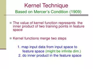
Kernel Technique. Based on Mercer’s Condition (1909). The value of kernel function represents the inner product of two training points in feature space Kernel functions merge two steps 1. map input data from input space to feature space (might be infinite dim.)

E N D
Kernel Technique Based on Mercer’s Condition (1909) • The value of kernel function represents the inner product of two training points in feature space • Kernel functions merge two steps 1. map input data from input space to feature space(might be infinite dim.) 2. do inner product in the feature space
is an integer: • Polynomial Kernel : ) (Linear Kernel : : • Gaussian (Radial Basis) Kernel represents the “similarity” -entryof More Examples of Kernel • The of data points and
Nonlinear 1-Norm Soft Margin SVM In Dual Form Linear SVM: Nonlinear SVM:
Solve the quadratic program for some : min , s. t. where , denotes or membership. 1-norm Support Vector MachinesGood for Feature Selection Equivalent to solve a Linear Program as follows:
min (QP) s. t. At the solution of(QP): Hence(QP)is equivalent to thenonsmooth SVM: where min SVM as anUnconstrained Minimization Problem • Change(QP)into an unconstrained MP • Reduce (n+1+m) variables to (n+1) variables
Smooth the Plus Function:Integrate Step function: Sigmoid function: p-function: Plus function:
in thenonsmooth • Replacing the plus function , gives ourSSVM: SVMby the smooth min • The solution ofSSVMconverges to the solution of goes to infinity. nonsmooth SVM as ) (Typically, SSVM: Smooth Support Vector Machine
The sequence generated by solving a quadratic approximation ofSSVM, converges to the unique solution of SSVMat a quadratic rate. Newton-Armijo Method: Quadratic Approximation of SSVM • Converges in 6 to 8 iterations • At each iteration we solve a linear system of: • n+1 equations in n+1 variables • Complexity depends ondimensionof input space • It might be needed to select a stepsize
Start with any . Having Newton-Armijo Algorithm stop if else : (i) Newton Direction : globally and quadratically converge to unique solution in a finite number of steps (ii) Armijo Stepsize : such that Armijo’s rule is satisfied
Replace by a nonlinear kernel : min • Each iteration solves m+1 linear equations in m+1 variables Nonlinear Smooth SVM Nonlinear Classifier: • Use Newton-Armijo algorithm to solve the problem • Nonlinear classifier depends on the data points with nonzero coefficients :
SSVM:A new formulation of support vector machine as a smooth unconstrained minimization problem • How to select parameters: Conclusion • An overview ofSVMs for classification • Can be solved by a fast Newton-Armijo algorithm • No optimization (LP, QP) package is needed • There are many important issues did not address this lecture such as: • How to solve conventional SVM? • How to deal with massive datasets?
x1 x2 xn Perceptron • Linear threshold unit (LTU) x0=1 w0 w1 w2 . . . i=0nwi xi g wn 1 if i=0nwi xi>0 o(xi)= -1 otherwise {
Possibilities for functiong Sign function Sigmoid (logistic) function Step function sign(x) = +1, if x > 0 -1, if x 0 step(x) = 1, if x> threshold 0, if x threshold (in picture above, threshold = 0) sigmoid(x) = 1/(1+e-x) Adding an extra input with activation x0 = 1 and weight wi, 0 = -T (called the bias weight) is equivalent to having a threshold at T. This way we can always assume a 0 threshold.
Using a Bias Weight to Standardize the Threshold 1 -T w1 x1 w2 x2 w1x1+ w2x2 < T w1x1+ w2x2 - T< 0
t=-1 t=1 o=1 w=[0.25 –0.1 0.5] x2 = 0.2 x1 – 0.5 o=-1 (x,t)=([2,1],-1) o=sgn(0.45-0.6+0.3) =1 (x,t)=([-1,-1],1) o=sgn(0.25+0.1-0.5) =-1 w=[0.2 –0.2 –0.2] w=[-0.2 –0.4 –0.2] (x,t)=([1,1],1) o=sgn(0.25-0.7+0.1) =-1 w=[0.2 0.2 0.2] -0.5x1+0.3x2+0.45>0 o = 1 Perceptron Learning Rule x2 x2 x1 x1 x2 x2 x1 x1
learning rate and the initial weight vector, bias: and let The Perceptron AlgorithmRosenblatt, 1956 Given a linearly separable training set and
The Perceptron Algorithm(Primal Form) Repeat: until no mistakes made within the for loop return: ? . What is
Let be a non-trivial training set, and let on is at most The Perceptron Algorithm ( STOP in Finite Steps ) Theorem (Novikoff) Suppose that there exists a vector and . Then the number of mistakes made by the on-line perceptron algorithm
The algorithm starts with an augmented weight vector and updates it at each mistake. Let be the augmented weight vector prior to the th mistake. The th update is performed when where is the point incorrectly classified by . Proof of Finite Termination Proof: Let
Update Rule of Perceotron Similarly,
Given a linearly separable training set and Repeat: until no mistakes made within the for loop return: The Perceptron Algorithm(Dual Form)
The number of updates equals: implies that the training point has been misclassified in the training process at least once. implies that removing the training point will not affect the final results • The training data only appear in the algorithm through the entries of the Gram matrix, which is defined below: What We Got in the Dual Form Perceptron Algorithm?
Reuters-2157821578 docs – 27000 terms, and 135 classes • 21578 documents • 1-14818 belong to training set • 14819-21578 belong to testing set • Reuters-21578 includes 135 categories by using ApteMod version of the TOPICS set • Result in 90 categories with 7,770 training documents and 3,019 testing documents
Preprocessing Procedures (cont.) • After Stopwords Elimination • After Porter Algorithm
Binary Text Classificationearn(+) vs. acq(-) • Select top 500 terms using mutual information • Evaluate each classifier using F-measure • Compare two classifiers using 10-fold paired-t test
Rejectwith 95% confidence level 10-fold Testing ResultsRSVM vs. Naïve Bayes There is no difference between RSVM and NB
Multi-Class SVMs • Combining into multi-class classifier • One-vs-Rest • Classes: in this class or not in this class • Positive training samples: data in this class • Negative training samples: the rest • K binary SVMs (k is the number of classes) • One-vs-One • Classes: in class one or in class two • Positive training samples: data in this class • Negative training samples: data in the other class • K(K-1)/2 binary SVM
Performance Measures • Precision and recall • F-measure , where TP is the number of true positive, FP is the number of false positive, and FN is the number of false negative.
Measures for Multi-class Classification (one vs. rest) • Macro-averaging: arithmetic average • Micro-averaging: averages the contingency (confusion) tables