Download
1 / 45
450 likes | 634 Views
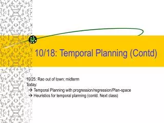
10/18: Temporal Planning (Contd). 10/25: Rao out of town; midterm Today: Temporal Planning with progression/regression/Plan-space Heuristics for temporal planning (contd. Next class). S et < pi,ti> of predicates pi and the time of their last achievement t i < t. Set of protected

E N D
10/18: Temporal Planning (Contd) 10/25: Rao out of town; midterm Today: Temporal Planning with progression/regression/Plan-space Heuristics for temporal planning (contd. Next class)
Set <pi,ti> of predicates pi and the time of their last achievement ti < t. Set of protected persistent conditions (could be binary or resource conds). Time stamp of S. Set of functions represent resource values. Event queue (contains resource as well As binary fluent events). State-Space Search:Search is through time-stamped states Review Search states should have information about -- what conditions hold at the current time slice (P,M below) -- what actions have we already committed to put into the plan (,Q below) S=(P,M,,Q,t) In the initial state, P,M, non-empty Q non-empty if we have exogenous events
Review Light-match Let current state S be P:{have_light@0; at_steps@0}; Q:{~have_light@15} t: 0 (presumably after doing the light-candle action) Applying cross_cellar to this state gives S’= P:{have_light@0; crossing@0}; :{have_light,<0,10>} Q:{at_fuse-box@10;~have_light@15} t: 0 Time-stamp Light-match Cross-cellar 15 10
“Advancing” the clock as a device for concurrency control To support concurrency, we need to consider advancing the clock How far to advance the clock? One shortcut is to advance the clock to the time of the next earliest event event in the event queue; since this is the least advance needed to make changes to P and M of S. At this point, all the events happening at that time point are transferred from Q to P and M (to signify that they have happened) This This strategy will find “a” plan for every problem—but will have the effect of enforcing concurrency by putting the concurrent actions to “align on the left end” In the candle/cellar example, we will find plans where the crossing cellar action starts right when the light-match action starts If we need slack in the start times, we will have to post-process the plan If we want plans with arbitrary slacks on start-times to appears in the search space, we will have to consider advancing the clock by arbitrary amounts (even if it changes nothing in the state other than the clock time itself). Review In the cellar plan above, the clock, If advanced, will be advanced to 15, Where an event (~have-light will occur) This means cross-cellar can either be done At 0 or 15 (and the latter makes no sense) ~have-light Light-match Cross-cellar Cross-cellar 15 10
Search Algorithm (cont.) • Goal Satisfaction: S=(P,M,,Q,t) G if <pi,ti> G either: • <pi,tj> P, tj < ti and no event in Q deletes pi. • e Q that adds pi at time te < ti. • Action Application: Action A is applicable in S if: • All instantaneous preconditions of A are satisfied by P and M. • A’s effects do not interfere with and Q. • No event in Q interferes with persistent preconditions of A. • A does not lead to concurrent resource change • When A is applied to S: • P is updated according to A’s instantaneous effects. • Persistent preconditions of A are put in • Delayed effects of A are put in Q. S=(P,M,,Q,t) [TLplan; Sapa; 2001]
Interference Clearly an overkill
Regression Search is similar… We can either work On R at tinf or R and Q At tinf-D(A3) R W X y • In the case of regression over durative actions too, the main generalization we need is differentiating the “advancement of clock” and “application of a relevant action” • Can use same state representation S=(P,M,,Q,t) with the semantics that • P and M are binary and resource subgoals needed at current time point • Q are the subgoals needed at earlier time points • are subgoals to be protected over specific intervals • We can either add an action to support something in P or Q, or push the clock backward before considering subgoals • If we push the clock backward, we push it to the time of the latest subgoal in Q • TP4 uses a slightly different representation (with State and Action information) Q A3:W A2:X A1:Y To work on have_light@<t1,t2>, we can either --support the whole interval directly with one action --or first split <t1,t2> to two subintervals <t1,t’> <t’,t2> and work on supporting have-light on both intervals [TP4; 1999]
Let current state S be P:{at_fuse_box@0} t: 0 Regressing cross_cellar over this state gives S’= P:{}; :{have_light,< 0 , -10>} Q:{have_light@ -10;at_stairs@-10} t: 0 Cross_cellar Have_light Notice that in contrast to progression, Regression will align the end points of Concurrent actions…(e.g. when we put in Light-match to support have-light)
Notice that in contrast to progression, Regression will align the end points of Concurrent actions…(e.g. when we put in Light-match to support have-light) Cross_cellar S’= P:{}; :{have_light,< 0 , -10>} Q:{have_light@-10;at_stairs@-10} t: 0 If we now decide to support the subgoal in Q Using light-match S’’=P:{} Q:{have-match@-15;at_stairs@-10} :{have_light,<0 , -10>} t: 0 Have_light Cross_cellar Have_light Light-match
PO (Partial Order) Search Involves LPsolving over Linear constraints (temporal constraints Are linear too); Waits for nonlinear constraints To become linear. Involves Posting temporal Constraints, and Durative goals Split the Interval into Multiple overlapping intervals [Zeno; 1994]
At_fusebox Have_light@t1 t1 I Cross_cellar G t2 at_fuse_box@G} Have_light@<t1,t2> t2-t1 =10 t1 < tG tI < t1
The ~have_light effect at t4 can violate the <have_light, t3,t1> causal link! Resolve by Adding T4<t3 V t1<t4 ~have-light t3 t4 Burn_match At_fusebox Have_light@t1 t1 I Cross_cellar G t2 at_fuse_box@G} Have_light@<t1,t2> t2-t1 =10 t1 < tG tI < t1 T4<tG T4-t3=15 T3<t1 T4<t3 V t1<t4
Notice that zeno allows arbitrary slack between the two actions ~have-light t3 t4 Burn_match At_fusebox Have_light@t1 t1 I Cross_cellar G t2 at_fuse_box@G} Have_light@<t1,t2> t2-t1 =10 t1 < tG tI < t1 T4<tG T4-t3=15 T3<t1 T4<t3 V t1<t4 T3<t2 T4<t3 V t2<t4 To work on have_light@<t1,t2>, we can either --support the whole interval directly by adding a causal link <have-light, t3,<t1,t2>> --or first split <t1,t2> to two subintervals <t1,t’> <t’,t2> and work on supporting have-light on both intervals
Tradeoffs: Progression/Regression/PO Planning for metric/temporal planning • Compared to PO, both progression and regression do a less than fully flexible job of handling concurrency (e.g. slacks may have to be handled through post-processing). • Progression planners have the advantage that the exact amount of a resource is known at any given state. So, complex resource constraints are easier to verify. PO (and to some extent regression), will have to verify this by posting and then verifying resource constraints. • Currently, SAPA (a progression planner) does better than TP4 (a regression planner). Both do oodles better than Zeno/IxTET. However • TP4 could be possibly improved significantly by giving up the insistence on admissible heuristics • Zeno (and IxTET) could benefit by adapting ideas from RePOP.
Multi-objective search • Multi-dimensional nature of plan quality in metric temporal planning: • Temporal quality (e.g. makespan, slack—the time when a goal is needed – time when it is achieved.) • Plan cost (e.g. cumulative action cost, resource consumption) • Necessitates multi-objective optimization: • Modeling objective functions • Tracking different quality metrics and heuristic estimation Challenge: There may be inter-dependent relations between different quality metric
Tempe Los Angeles Phoenix Example • Option 1: Tempe Phoenix (Bus) Los Angeles (Airplane) • Less time: 3 hours; More expensive: $200 • Option 2: Tempe Los Angeles (Car) • More time: 12 hours; Less expensive: $50 • Given a deadline constraint (6 hours) Only option 1 is viable • Given a money constraint ($100) Only option 2 is viable
Solution Quality in the presence of multiple objectives • When we have multiple objectives, it is not clear how to define global optimum • E.g. How does <cost:5,Makespan:7> plan compare to <cost:4,Makespan:9>? • Problem: We don’t know what the user’s utility metric is as a function of cost and makespan.
Solution 1: Pareto Sets • Present pareto sets/curves to the user • A pareto set is a set of non-dominated solutions • A solution S1 is dominated by another S2, if S1 is worse than S2 in at least one objective and equal in all or worse in all other objectives. E.g. <C:4,M9> dominated by <C:5;M:9> • A travel agent shouldn’t bother asking whether I would like a flight that starts at 6pm and reaches at 9pm, and cost 100$ or another ones which also leaves at 6 and reaches at 9, but costs 200$. • A pareto set is exhaustive if it contains all non-dominated solutions • Presenting the pareto set allows the users to state their preferences implicitly by choosing what they like rather than by stating them explicitly. • Problem: Exhaustive Pareto sets can be large (exponentially large in many cases). • In practice, travel agents give you non-exhaustive pareto sets, just so you have the illusion of choice • Optimizing with pareto sets changes the nature of the problem—you are looking for multiple rather than a single solution.
Solution 2: Aggregate Utility Metrics • Combine the various objectives into a single utility measure • Eg: w1*cost+w2*make-span • Could model grad students’ preferences; with w1=infinity, w2=0 • Log(cost)+ 5*(Make-span)25 • Could model Bill Gates’ preferences. • How do we assess the form of the utility measure (linear? Nonlinear?) • and how will we get the weights? • Utility elicitation process • Learning problem: Ask tons of questions to the users and learn their utility function to fit their preferences • Can be cast as a sort of learning task (e.g. learn a neual net that is consistent with the examples) • Of course, if you want to learn a true nonlinear preference function, you will need many many more examples, and the training takes much longer. • With aggregate utility metrics, the multi-obj optimization is, in theory, reduces to a single objective optimization problem • *However* if you are trying to good heuristics to direct the search, then since estimators are likely to be available for naturally occurring factors of the solution quality, rather than random combinations there-of, we still have to follow a two step process • Find estimators for each of the factors • Combine the estimates using the utility measure THIS IS WHAT IS DONE IN SAPA
Sketch of how to get cost and time estimates • Planning graph provides “level” estimates • Generalizing planning graph to “temporal planning graph” will allow us to get “time” estimates • For relaxed PG, the generalization is quite simple—just use bi-level representation of the PG, and index each action and literal by the first time point (not level) at which they can be first introduced into the PG • Generalizing planning graph to “cost planning graph” (i.e. propagate cost information over PG) will get us cost estimates • We discussed how to do cost propagation over classical PGs. Costs of literals can be represented as monotonically reducing step functions w.r.t. levels. • To estimate cost and time together we need to generalize classical PG into Temporal and Cost-sensitive PG • Now, the costs of literals will be monotonically reducing step functions w.r.t. time points (rather than level indices) • This is what SAPA does
SAPA approach • Using the Temporal Planning Graph (Smith & Weld) structure to track the time-sensitive cost function: • Estimation of the earliest time (makespan) to achieve all goals. • Estimation of the lowest cost to achieve goals • Estimation of the cost to achieve goals given the specific makespan value. • Using this information to calculate the heuristic value for the objective function involving both time and cost • Involves propagating cost over planning graphs..
Heuristics in Sapa are derived from the Graphplan-style bi-level relaxed temporal planning graph (RTPG) Progression; so constructed anew for each state..
A B Person Airplane Person t=0 tg Load(P,A) Unload(P,A) Fly(A,B) Fly(B,A) Unload(P,B) Init Goal Deadline Note: Bi-level rep; we don’t actually stack actions multiple times in PG—we just keep track the first time the action entered Relaxed Temporal Planning Graph RTPG is modeled as a time-stamped plan! (but Q only has +ve events) • Relaxed Action: • No delete effects • May be okay given progression planning • No resource consumption • Will adjust later • while(true) • forallAadvance-time applicable in S • S = Apply(A,S) • Involves changing P,,Q,t • {Update Q only with positive • effects; and only when there is no other earlier event giving that effect} • ifSG then Terminate{solution} • S’ = Apply(advance-time,S) • if (pi,ti) G such that • ti < Time(S’) and piS then • Terminate{non-solution} • elseS = S’ • end while; Deadline goals
Heuristics directly from RTPG A D M I S S I B L E • For Makespan: Distance from a state S to the goals is equal to the duration between time(S) and the time the last goal appears in the RTPG. • For Min/Max/Sum Slack: Distance from a state to the goals is equal to the minimum, maximum, or summation of slack estimates for all individual goals using the RTPG. • Slack estimate is the difference between the deadline of the goal, and the expected time of achievement of that goal. Proof: All goals appear in the RTPG at times smaller or equal to their achievable times.
A B Person Airplane Person t=0 tg Load(P,A) Unload(P,A) Fly(A,B) Fly(B,A) Unload(P,B) Init Goal Deadline Heuristics from Relaxed Plan Extracted from RTPG RTPG can be used to find a relaxed solution which is then used to estimate distance from a given state to the goals Sum actions: Distance from a state S to the goals equals the number of actions in the relaxed plan. Sum durations: Distance from a state S to the goals equals the summation of action durations in the relaxed plan.
Resource-based Adjustments to Heuristics Resource related information, ignored originally, can be used to improve the heuristic values Adjusted Sum-Action: h = h + R (Con(R) – (Init(R)+Pro(R)))/R Adjusted Sum-Duration: h = h + R [(Con(R) – (Init(R)+Pro(R)))/R].Dur(AR) Will not preserve admissibility
Tempe Los Angeles Phoenix Drive-car(Tempe,LA) Heli(T,P) Airplane(P,LA) Shuttle(T,P) t = 10 t = 0 t = 0.5 t = 1 t = 1.5 The (Relaxed) Temporal PG
Tempe L.A Phoenix Time-sensitive Cost Function cost • Standard (Temporal) planning graph (TPG) shows the time-related estimates e.g. earliest time to achieve fact, or to execute action • TPG does not show the cost estimates to achieve facts or execute actions $300 $220 $100 0 1.5 2 10 time Drive-car(Tempe,LA) Airplane(P,LA) Heli(T,P) Shuttle(Tempe,Phx): Cost: $20; Time: 1.0 hour Helicopter(Tempe,Phx): Cost: $100; Time: 0.5 hour Car(Tempe,LA): Cost: $100; Time: 10 hour Airplane(Phx,LA): Cost: $200; Time: 1.0 hour Shuttle(T,P) t = 10 t = 0 t = 0.5 t = 1 t = 1.5
Drive-car(Tempe,LA) Tempe Airplane(P,LA) Hel(T,P) Airplane(P,LA) Shuttle(T,P) L.A Phoenix t = 10 t = 0 t = 0.5 t = 1 t = 1.5 t = 2.0 0.5 Estimating the Cost Function Shuttle(Tempe,Phx): Cost: $20; Time: 1.0 hour Helicopter(Tempe,Phx): Cost: $100; Time: 0.5 hour Car(Tempe,LA): Cost: $100; Time: 10 hour Airplane(Phx,LA): Cost: $200; Time: 1.0 hour $300 $220 $100 $20 time 0 1 1.5 2 10 Cost(At(LA)) Cost(At(Phx)) = Cost(Flight(Phx,LA))
Observations about cost functions ADDED • Because cost-functions decrease monotonically, we know that the cheapest cost is always at t_infinity (don’t need to look at other times) • Cost functions will be monotonically decreasing as long as there are no exogenous events • Actions with time-sensitive preconditions are in essence dependent on exogenous events (which is why PDDL 2.1 doesn’t allow you to say that the precondition must be true at an absolute time point—only a time point relative to the beginning of the action • If you have to model an action such as “Take Flight” such that it can only be done with valid flights that are pre-scheduled (e.g. 9:40AM, 11:30AM, 3:15PM etc), we can model it by having a precondition “Have-flight” which is asserted at 9:40AM, 11:30AM and 3:15PM using timed initial literals) • Becase cost-functions are step funtions, we need to evaluate the utility function U(makespan,cost) only at a finite number of time points (no matter how complex the U(.) function is. • Cost functions will be step functions as long as the actions do not model continuous change (which will come in at PDDL 2.1 Level 4). If you have continuous change, then the cost functions may change continuously too
Cost Propagation • Issues: • At a given time point, each fact is supported by multiple actions • Each action has more than one precondition • Propagation rules: • Cost(f,t) = min {Cost(A,t) : f Effect(A)} • Cost(A,t) = Aggregate(Cost(f,t): f Pre(A)) • Sum-propagation: Cost(f,t) • The plans for individual preconds may be interacting • Max-propagation: Max {Cost(f,t)} • Combination: 0.5 Cost(f,t) + 0.5 Max {Cost(f,t)} Can’t use something like set-level idea here because That will entail tracking the costs of subsets of literals Probably other better ideas could be tried
Termination Criteria cost • Deadline Termination: Terminate at time point t if: • goal G: Dealine(G) t • goal G: (Dealine(G) < t) (Cost(G,t) = • Fix-point Termination: Terminate at time point t where we can not improve the cost of any proposition. • K-lookahead approximation: At t where Cost(g,t) < , repeat the process of applying (set) of actions that can improve the cost functions k times. $300 $220 $100 0 1.5 2 10 time Earliest time point Cheapest cost Drive-car(Tempe,LA) Plane(P,LA) H(T,P) Shuttle(T,P) t = 0 0.5 1.5 1 t = 10
Heuristic estimation using the cost functions The cost functions have information to track both temporal and cost metric of the plan, and their inter-dependent relations !!! • If the objective function is to minimize time: h = t0 • If the objective function is to minimize cost: h = CostAggregate(G, t) • If the objective function is the function of both time and cost O = f(time,cost) then: h = min f(t,Cost(G,t))s.t.t0 t t Eg:f(time,cost) = 100.makespan + Costthen h = 100x2 + 220 at t0 t = 2 t cost $300 $220 $100 0 t0=1.5 2 t = 10 time Cost(At(LA)) Earliest achieve time: t0 = 1.5 Lowest cost time: t = 10
Heuristic estimation by extracting the relaxed plan • Relaxed plan satisfies all the goals ignoring the negative interaction: • Take into account positive interaction • Base set of actions for possible adjustment according to neglected (relaxed) information (e.g. negative interaction, resource usage etc.) Need to find a good relaxed plan (among multiple ones) according to the objective function
Heuristic estimation by extracting the relaxed plan cost • General Alg.: Traverse backward searching for actions supporting all the goals. When A is added to the relaxed plan RP, then: Supported Fact = SF Effects(A) Goals = SF \ (G Precond(A)) • Temporal Planning with Cost: If the objective function is f(time,cost), then A is selected such that: f(t(RP+A),C(RP+A)) + f(t(Gnew),C(Gnew)) is minimal(Gnew = (G Precond(A)) \ Effects) • Finally, using mutex to set orders between A and actions in RP so that less number of causal constraints are violated $300 $220 $100 0 t0=1.5 2 t = 10 time Tempe L.A Phoenix f(t,c) = 100.makespan + Cost
Adjusting the Heuristic Values Ignored resource related information can be used to improve the heuristic values (such like +ve and –ve interactions in classical planning) Adjusted Cost: C = C + R (Con(R) – (Init(R)+Pro(R)))/R * C(AR) Cannot be applied to admissible heuristics
Partialization Example A position-constrained plan with makespan 22 A1(10) gives g1 but deletes p A3(8) gives g2 but requires p at start A2(4) gives p at end We want g1,g2 A1 A2 A3 p Order Constrained plan The best makespan dispatch of the order-constrained plan A2 g2 A3 G A2 A3 14+e A1 A1 g1 There could be multiple O.C. plans because of multiple possible causal sources. Optimization will involve Going through them all. [et(A1) <= et(A2)] or [st(A1) >= st(A3)] [et(A2) <= st(A3) ….
Problem Definitions • Position constrained (p.c) plan: The execution time of each action is fixed to a specific time point • Can be generated more efficiently by state-space planners • Order constrained (o.c) plan: Only the relative orderings between actions are specified • More flexible solutions, causal relations between actions • Partialization: Constructing a o.c plan from a p.c plan t1 t2 t3 Q R Q R R R G G R R Q Q {Q} {Q} {G} {G} p.c plan o.c plan
Validity Requirements for a partialization • An o.c plan Poc is a valid partialization of a valid p.c plan Ppc, if: • Poc contains the same actions as Ppc • Poc is executable • Pocsatisfies all the top level goals • (Optional) Ppcis a legal dispatch (execution) of Poc • (Optional) Contains no redundant ordering relations redundant X P P Q Q
Greedy Approximations • Solving the optimization problem for makespan and number of orderings is NP-hard (Backstrom,1998) • Greedy approaches have been considered in classical planning (e.g. [Kambhampati & Kedar, 1993], [Veloso et. al.,1990]): • Find a causal explanation of correctness for the p.c plan • Introduce just the orderings needed for the explanation to hold
Modeling greedy approaches as value ordering strategies • Variation of [Kambhampati & Kedar,1993] greedy algorithm for temporal planning as value ordering: • Supporting variables: SpA = A’ such that: • etpA’ < stpAin the p.c plan Ppc • B s.t.: etpA’ < etpB < stpA • C s.t.: etpC < etpA’and satisfy two above conditions • Ordering and interference variables: • pAB = < ifetpB < stpA ; pAB = > ifstpB > stpA • rAA’= < if etrA < strA’inPpc; rAA’= > if strA > etrA’inPpc; rAA’= other wise. Key insight:We can capture many of the greedy approaches as specific value ordering strategies on the CSOP encoding
Empirical evaluation • Objective: • Demonstrate that metric temporal planner armed with our approach is able to produce plans that satisfy a variety of cost/makespan tradeoff. • Testing problems: • Randomly generated logistics problems from TP4 (Hasslum&Geffner) Load/unload(package,location):Cost = 1; Duration = 1; Drive-inter-city(location1,location2):Cost = 4.0; Duration = 12.0; Flight(airport1,airport2):Cost = 15.0; Duration = 3.0; Drive-intra-city(location1,location2,city):Cost = 2.0; Duration = 2.0;