Download
1 / 6
60 likes | 182 Views
Our final topics this semester are density estimation and nonparametric regression in sections 10.1 and 10.2...

E N D
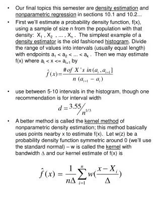
Our final topics this semester are density estimation and nonparametric regression in sections 10.1 and 10.2... • First we’ll estimate a probability density function, f(x), using a sample of size n from the population with that density: X1 , X2 , ... , Xn . The simplest example of a density estimator is the old fashioned histogram. Divide the range of values into intervals (usually equal length) with endpoints a1 < a2 < ... < ak . Then we may estimate f(x) where ai < x <= ai+1 by • use between 5-10 intervals in the histogram, though one recommendation is for interval width • A better method is called the kernel method of nonparametric density estimation; this method basically uses points nearby x to estimate f(x). Let w(z) be a probability density function symmetric around 0 (we’ll use the standard normal) – w is called the kernel with bandwidth D and our kernel estimate of f(x) is
one suggestion for choosing the bandwidth is to let • as with histograms, smaller values of delta will yield estimates that fit more details in the data, while larger values will lead to smoother estimates – our textbook says “one should not be timid about varying delta” – try several values around the suggested values to see which gives a better fitting estimate... • two other methods of bandwidth selection are: • cross-validation (hcv – see below) • Sheather-Jones approach (hsj – see below) • besides the R function density which gives smooth estimates of a univariate distribution of data, there is another package in R that adds several functions of interest to us, including the two bandwidth selectors above. It is called sm (for “smoothing”). Load it in R by library(sm) - if your version of R doesn’t have it available, go to CRAN and download it... I’ll show you how in class • another function in the base package of R that also helps with density estimation is called rug... see the help file and try it on the faithful data...
The use of regression methods to model two-dimensional data is widespread – but the usual parametric assumptions of normality are often not applicable and nonparametric regression attempts to fill the gap... also, we sometimes just want to use a smooth curve (rather than a line) to guide our exploration of a scatterplot • The basic idea is to use the (x,y) data to fit a more general function than a linear one: fit y = m(x) + e instead of y = ax + b + e . Here y is the response, x is the explanatory variable, m(x) is the (unknown) underlying function relating x to y, and e is assumed to be an independent error term with mean=0 and s.d.=s . • As density estimation trys to “average” counts of data locally, so does nonparametric regression; i.e., the estimated curve at x is made of “averages” of the response in a neighborhood of x – local regression. • There are many approaches... a simple kernel method is called the local mean estimator
Here’s the local mean estimator (w is the kernel function, h is the bandwidth – frequently assume w is N(0,h)) • Note that this is just a weighted mean of the response values, the highest weights being assigned to those values of the data closest to the x where m(x) is being estimated. • As before, the smoothing parameter (bandwidth) h controls the width of the kernel and hence the amount of smoothing. When h is the s.d. of a normal kernel, observations within about 3h of x will contribute to the estimate. As h increases, some characteristics of the relationship between x and y are missed and as h decreases, the estimate tracks the data too closely and the result is a “wiggly” estimate. • Another more powerful regression estimator is the local linear estimator – it is implemented in R in the sm package as sm.regression(x,y) and in a similar function called loess in R... we’ll see now how these work...
The local linear regression function sm.regression uses the usual least squares fitting with weights applied by the kernel function with bandwidth h... find the values of a and b that minimize • In sm.regression, the default kernel is the normal kernel with s.d.=h and mean=0. Note that this can be considered as an extension of the usual least squares regresssion in the sense that as h gets larger and larger, the local linear regression approaches usual least squares regression (lm(x,y) = sm.regression(x,y) when h is very large) • The following page gives some R code that will implement the sm.regression function on a dataset of Bowman and Azzalini’s involving carbon dating... Their provide.data function puts the dataset into the workspace...
provide.data(radioc) #Cal.age is the “true” calendar age, #Rc.age is the carbon dated age par(mfrow=c(1,2)) plot(Cal.age,Rc.age); abline(0,1,lty=2) #note the 2 ages don’t agree #look at those points whose calendar #age is between 2000 and 3000 ind=(Cal.age>2000 & Cal.age<3000) #this is a logical function, TRUE when #both are true ind #now subset wrt ind and do l.s. and #local linear regression and compare... cal.age=Cal.age[ind]; rc.age=Rc.age[ind] sm.regression(cal.age,rc.age,h=30) sm.regression(cal.age,rc.age,h=1000, lty=2,add=T)