Designing Observers for Full State Feedback Control in Linear Systems
In control system design, full state feedback is essential, yet we often lack access to all state variables, necessitating the use of observers. This lecture explores the construction of observers for single-input single-output (SISO) systems. We focus on estimating unmeasured state variables using available output data, minimizing the difference between actual and estimated states. This involves techniques like pole placement and ensures system stability. The interplay between controllability and observability is highlighted, emphasizing the role of observer gain in achieving desired system performance.

Designing Observers for Full State Feedback Control in Linear Systems
E N D
Presentation Transcript
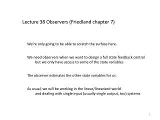
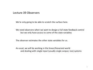
Lecture 39 Observers We’re only going to be able to scratch the surface here. We need observers when we want to design a full state feedback control but we only have access to some of the state variables The observer estimates the other state variables for us. As usual, we will be working in the linear/linearized world and dealing with single input (usually single output, too) systems
and we’ll suppose for the moment that all we want to do is make x go to zero
The dynamical system x u y c b A
We can design a control law (if the system is controllable) that will do that but we cannot implement this unless we know all the components of the state vector
Suppose that all we know is an output y, a scalar for an SISO system We use y, the control and an artificial dynamical system to find an estimate for x This artificial system is called an observer
The observer u y k
We select k and the carat matrices to minimize the difference between x and its estimate.
This is a different error from that we used for tracking For tracking we asked that x —> xr and e was the difference between x and xr We suppose here that xr is 0 We want to make x go to 0 We cannot measure x, so we have to estimate it Our error here is the difference between x and its estimate
So we have two goals: make x go to zero make the difference between x and xr go to zero These are, in some sense, the same goals for this problem but we need to treat them as separate to be general enough for other problems Let’s start by working on the error, the difference between the two states
As usual we want to construct a system for the evolution of the estimate error and, of course, make the estimate error go to zero We eliminate the explicit appearance of the estimate using the error definition
copy the equation and rearrange e will go to zero if I get rid of the contributions from x and u and make sure the new matrix is stable This becomes a pole placement exercise
Take a look at the pole placement exercise I know A and c, but I do not know k, so the idea is to place poles by finding k These are the poles that will drive the estimate error to zero they do not drive x to zero — that takes a separate effort
finding k The substitutions give and the error will vanish of the eigenvalues have negative real parts. We need to find k such that this is so. We have two questions: Is this possible? If so, how do we do it?
finding k For our SISO system the k vector is a column and the system looks like We can make this look like something we already know how to do The eigenvalues of the transpose of a matrix are the same as those of the original matrix
finding k the pattern for finding k now looks just like the pattern for finding g AT plays the role of A, c that of b and k that of g and we can follow the same procedure
finding k We have the analog of the controllability theorem The observability theorem We can build an observer if det(N) ≠ 0.
finding k The rank of N is the same as the rank of NT, and the observability condition is often expressed in terms of NT We cannot make an effective observer if this matrix is not of full rank We work with the original N matrix to build an observer of an observable system Observability is expressed in terms of A and c; Controllability is expressed in terms of A and b
finding k We wind up with a companion form, for which we can place poles and then map the whole thing back again We are mapping back from a companion form and we can use the same technique At this point we have designed the observer, and we can put the system and the observer together
x u y c b A y k connection
Now we can go back to finding the gain matrix We find g in the usual way by transforming the problem into z space (the last row of Q-1) This is not the same T that we used for k
A1 is in companion form (here’s a 6 x 6 to remind you of the pattern)
Put the package together The characteristic polynomial
Equate coefficients to those of the desired polynomial to find the zgains Map the z gains back to x space for calculation The new wrinkle for this problem is that we don’t know x We have to fit this into the double system we explored earlier
x y c u b A y k
FINAL PICTURE u x c b y A k
How does this actually work? We use the estimate to define the control that we designed to stabilize x We have a pair of coupled dynamical systems we let The calculation of g and k are independent
What do you actually do to simulate this? I’ll just consider the linear problem today Integrate these two vector equations simultaneously — they are coupled
Summary for an SISO system to control this we put We find g the way we already now how to do: use the companion form algorithm but we don’t know all of x, just y = cTx, so we must put and we need to figure out an estimate for x which we do by constructing an observer
The estimate is supposed to be driven by both u and y We construct the dynamics of the estimate by asking that the difference between x and its estimate go to zero We found that gives and we find k following a routine just like that to find g Summary picture on the next slide
FINAL PICTURE u x c b y A k
Let’s try to look at this in a simple context: the servo motor We’ll do something more complicated later All I’m going to ask it to do is go back to the neutral position so I don’t have to worry about tracking I need equations, and I need to find the usual gains g and the new vector k
Find g A is already in companion form, and b is almost there. I would not bother with the companion form in real life, but . . .
Compare the characteristic polynomials Equating the coefficients of the polynomials gives us
I need to map the gains back to x space: gT = g’TT We find that k works about the same way
finding k We can copy the second order motion equations from Lecture 24 where and then
finding k Pick a generic c and calculate N We can admit c2 = 0, but we must be able to measure q. Let’s take c1 = 1 and c2 = 0: we measure the angle only
finding k This is different from the previous T
finding k And we have the characteristic polynomial for the ks We see that k’1 = s1s2 and k’2 = -KG – s1 – s2 If we put these poles at -1 we’ll get
We have to map these back as well, using the T for this transformation so that becomes
Let’s see if we can use this to move the servo π/2 These results are for the poles the same for both: -1 ±j