Download
1 / 6
60 likes | 204 Views
Monitoring Trends in Atmospheric Water Vapor Require Increasing Frequency of Measurements David Whiteman (613.1), Kevin Vermeesch (SSAI) Luke Oman (613.3), Elizabeth Weatherhead (CIRES, U. Colorado).

E N D
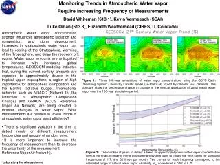
Monitoring Trends in Atmospheric Water VaporRequire Increasing Frequency of Measurements David Whiteman (613.1), Kevin Vermeesch (SSAI) Luke Oman (613.3), Elizabeth Weatherhead (CIRES, U. Colorado) • Atmospheric water vapor concentration strongly influences atmospheric radiation and composition, and storm development. Increases in stratospheric water vapor can lead to cooling of the Stratosphere, warming of the Troposphere, and delay the recovery of ozone, Water vapor amounts are anticipated to increase with increasing global temperatures. GEOSCCM modeling indicates that, during the current century, amounts are expected to approximately double in the tropical upper troposphere, a region of high importance for atmospheric composition and the Earth’s radiative budget. International networks such as NDACC (Network for the Detection of Atmospheric Composition Change) and GRAUN (GCOS Reference Upper Air Network) are being created to monitor changes in water vapor. What measurements are needed to reveal trends in atmospheric water vapor most efficiently? • There is significant variation in the time to detect trends for different measurement frequencies and amount of random error. • It is more important to increase the frequency of measurement than to decrease the uncertainty of the measurement. • Reference Upper Air Network). Figure 1: Three 100-year simulations of water vapor concentrations using the GSFC Earth Observing System Chemistry Climate Model (GEOSCCM) forced by different SST datasets. The contours show the percentage change in change in the vertical distribution of zonal mean water vapor over the 100-year simulation period. Figure 2: The number of years to detect a trend in upper tropospheric water vapor concentration versus the total uncertainty in the measurement system used to create the time series for sampling frequencies of 1,7, and 30 times per month. Two curves for each frequency correspond to the estimated range of natural water vapor variability, σA, considered is 0.56 to 0.75. Laboratory for Atmospheres
Name: David Whiteman, NASA/GSFC, Code 613.1 E-mail: david.n.whiteman@nasa.gov Phone: 301-614-6703 References: Whiteman, D. N., K. Vermeesch, L. Oman, E. Weatherhead, 2011: The relative importance of accuracy, random error, and observation frequency in detecting trends in upper tropospheric water vapor, Journal of Geophysical Research, in press. Oman, L, D. Waugh, S. Pawson, R. Stolarski, J.E. Nielsen, 2008: Understanding the Changes of Stratospheric Water Vapor in Coupled Chemistry–Climate Model Simulations, J. Atmos. Sciences, vol 65, p. 3278 Data Sources: Goddard Earth Observing System Chemistry Climate Model (GEOSCCM) simulations using Intergovernmental Panel on Climate Change (IPCC) greenhouse gas scenarios, and Department of Energy radiosonde data. Technical Description of Figures: Figure 1: The anticipated trend in water vapor amounts, calculated based on annual means, using the GSFC Earth Observing System Chemistry Climate Model (GEOSCCM) along with the International Panel on Climate Change (IPCC) greenhouse gas scenarios [IPCC, 2000] and 3 different SST simulations. Two simulations were run using the IPCC Special Report on Emission Scenarios (SRES) A1B greenhouse gas scenario. The runs differ in the SST and sea ice boundary conditions used. The first one used was the Hadley Centre climate model (HadGEM1) which has a larger than average climate sensitivity. The second was the Community Climate System Model version 3 (CCSM3) which has a lower than average climate sensitivity. The runs were conducted for the IPCC Fourth Assessment Report and the SST and sea ice output was used in GEOSCCM. An additional simulation was conducted using the IPCC SRES A2 greenhouse gas scenario with only CCSM3 SST and sea ice boundary conditions. This represents a higher-end emissions scenario. Figure 2: The figure shows the time to detect trends in upper tropospheric (200-hPa) water vapor for sampling frequencies of 1, 7, and 30 times per month and instrumental uncertainties ranging from 0% - 100% using the statistical tools developed by Tiao et al and Weatherhead et al. There are two curves for each sampling frequency corresponding to the estimated range of atmospheric noise (σA) of 0.56-0.75, based on analysis of radiosonde data. The predictions based on intermediate values of atmospheric noise are indicated by the shaded regions in the figure. For a perfect measurement system, i.e., one with no instrumental uncertainty, that provides measurements of upper tropospheric water vapor (200 hPa) on a daily basis, the time to detect trends ranges between approximately 12-15 years depending on the amount of atmospheric noise. The lower the atmospheric noise, the smaller the number of years to detect the trend. A daily time series of water vapor measurements created using an instrument possessing total noise of 50% increases the estimated range of times to detect trends by about 2-3 years to approximately 15-17 years. The larger increase corresponds to the assumption of lower atmospheric noise. By contrast, a time series created by a perfect measurement system operating 7 times per month will need to extend from 16-22 years to detect the same trend. Once monthly measurements will require a minimum of 35-42 years to reveal the trend. Scientific significance: Water vapor is important to atmospheric chemistry, radiation, dynamics, and cloud development. For example, increases in stratospheric water vapor can lead to cooling of the stratosphere, warming of the troposphere (Forster and Shine, 2002), and delay the recovery of ozone (Shindell, 2001; Weatherhead and Andersen, 2006). Solomon et al. (2010) have recently shown that decreases in lower stratospheric water vapor have slowed the rate of global surface temperature increase over the last decade. Trends in upper tropospheric water vapor concentrations and temperature will influence cirrus cloud frequency and composition. For these reasons and others, significant effort has been put into both measurements and modeling of UT/LS water vapor to assess long term trends in water vapor concentrations and thus address the consequences of changes in UT/LS water vapor amounts. Relevance for future science and relationship to Decadal Survey: Water vapor plays important roles in many atmospheric processes. Accurate profiling of water vapor is needed to determine how water vapor amounts are changing and what affects this has on the atmospheric system. Upcoming decadal survey missions such as The Precipitation and All-weather Temperature and Humidity (PATH) are tasked with quantifying the profile of water vapor in the atmosphere in the microwave region. Current missions such as AIRS and TES are quantifying water vapor profiles using Hyperspectral techniques in the IR. Laboratory for Atmospheres
Reduction of aerosol absorption in Beijing since 2007 from MODIS and AERONET A. Lyapustin, A. Smirnov, B. Holben, R. Kahn, M. Chin, D. Streets et al., Code 613.2, NASA GSFC The Multi-Angle Implementation of Atmosphe- ric Correction (MAIAC) is a new MODIS algo-rithm providing aerosol and land reflectance properties. Validation of MAIAC AOT with AERONET data over Beijing, China, indicates two distinct periods: prior to ∼March 2007 (period I), MAIAC underestimates AOT by 10–20% at peak values. This bias mostly disappears in period II (Figs. 1-2). The regression slope, which is strongly controlled by absorption, increases from 0.94 to 0.99 for Terra, and from 0.91 to 1.0 for Aqua between periods I and II. Because MAIAC used the same aerosol model for the entire time period, this points to a change in aerosol properties. By matching regression slopes in two periods, we assessed an increase in the single scattering albedo (SSA) by ~0.01. An analysis of AERONET data for Beijing showed a negligible change in effective particle size, and an increase in SSA by 0.02 over 9 years at 88% confidence level (Fig.3). Our analysis links this change to the reduction of the local black carbon emissions due to broad scale measures of Chinese government to improve air quality in advance of the 2008 Olympic Games and a recession of 2008-2009 [Lyapustin et al., 2011]. This result is confirmed by the long-term chemical composition analysis [Okuda et al., 2011] and IASI CO data (Fig.4). MODIS Aqua Figure 1:Time series of MAIAC and AERONET AOT data over Beijing at 0.47 m, for ∼9 years of MODIS Aqua. The arrow indicates the approximate boundary between periods I and II. Figure 2:Time series difference plots (AERONET ‐ MAIAC AOT)0.47 for moderate‐ to‐high atmospheric opacity (AERONET AOT >0.4) over Beijing. Figure 3 (left):Time series plot of AERONET single scattering albedo for the Beijing site. Points represent monthly averaged values. Figure 4 (bottom):Time series plot of IASI CO over Beijing. Points represent monthly mean values. The blue lines show CO emission reduction in period II. Period II Period I Laboratory for Atmospheres
Name: Alexei Lyapustin, NASA/GSFC Code 613.2E-mail: Alexei.I.Lyapustin@nasa.govPhone: 301-614-5998 References: Lyapustin, A., et al. (2011), Reduction of aerosol absorption in Beijing since 2007 from MODIS and AERONET, Geophys. Res. Lett., 38, L10803, doi:10.1029/2011GL047306. Okuda, T., et al. (2011), The impact of the pollution control measures for the 2008 Beijing Olympic Games on the chemical composition of aerosols, Atmos. Environ., 45, 2789–2794, doi:10.1016/j.atmosenv.2011.01.053. Data Sources: MODIS Level 1B data, AERONET Level 2 aerosol product, IASI Level 2 CO product. Technical Description of Figures: Figure 1:A time series of MAIAC and AERONET AOT data over Beijing at 0.47 m, for ∼9 years of MODIS Aqua. MAIAC AOT (black dots) is systematically lower than AERONET AOT (red dots) during period I. This bias disappears in period II indicating change in aerosol properties. Figure 2: The difference plot AERONET AOT ‐ MAIAC AOT for moderate‐to‐high atmospheric opacity (AERONET AOT >0.4) over Beijing from MODIS Aqua. Similarly to Figure 1, this figure shows a systematic negative bias of MAIAC AOT during 2002 – mid-2007 with respect to AERONET measurements. This bias largely disappears after mid-2007. Figure 3: The time series plot of AERONET single scattering albedo (SSA) for the Beijing site showing statistically significant increase of SSA by ~0.02 in 9 years. Figure 4. The time series of IASI CO over Beijing showing CO emission reduction in period II relative to period I. Scientific significance: Current satellite retrievals have very limited ability to evaluate aerosol absorption from multi-angle (MISR) or UV (OMI) measurements. In this work, we used a combination of MODIS and AERONET data and demonstrated a measurable reduction of the aerosol absorption over Beijing during 2007–2010 compared to the previous five years, most probably caused by the regulation of BC emissions. Two independent methods based on the time series analysis of a) MODIS/AERONET AOT data, and b) AERONET SSA data, give similar results which are in qualitative agreement with in situ chemical composition analysis [Okuda et al., 2011] and IASI CO data. The timing of these changes is correlated with expansive measures adopted by the Chinese government to improve air quality in Beijing in advance of the 2008 Olympic Games. Relevance for future science and relationship to Decadal Survey: (1)Currently, large uncertainties in climate modeling exist because of the complexity of aerosol processes and incomplete understanding of their interactions with the climate system [IPCC, 2007]. Aerosol absorption is one of the most important and least known climate-forming factors. A detection and characterization of trends in anthropogenic aerosol absorption is critical to improve our understanding of aerosol radiative and climate effects. The importance of studying this interaction is highlighted in the Decadal Survey and is a goal for future NASA missions such as GLORY and ACE. (2) The detected reduction of aerosol absorption is important for the modeling community as existing models predict increase in BC emissions based on emissions inventories. Laboratory for Atmospheres
Destruction of Mesospheric Arctic Ozone Caused by Solar Protons in January 2005 Charles Jackman (Code 613.3, NASA GSFC) and Eric Fleming (SSAI and Code 613.3, NASA GSFC) EOS Aura Solar eruptions in early 2005 led to a substantial barrage of charged particles on the Earth’s polar atmosphere during the January 16-21 period. Most of these charged particles were protons, thus the term “Solar Proton Event (SPE)” has been used to describe this phenomenon. The solar protons created hydrogen- containing compounds, which led to the polar ozone destruction. We have used the Aura Microwave Limb Sounder (MLS) observations to quantify the changes in the hydroxyl radical (OH), hydrogen dioxide (HO2), and ozone due to these SPEs. The atmospheric changes in OH, HO2, and ozone for the latitude band 60-82.5oN shown in Figure 1 are all relative to the quiet January 1-14, 2005 time period, which contained no SPEs. Fairly substantial OH enhancements (up to 4 ppbv) and HO2 enhancements (up to 0.8 ppbv) were caused by the SPEs. To the best of our knowledge, this is the first time that SPE-caused HO2 measured increases have been reported. The SPE-caused mesospheric ozone decreases (up to 80%, area outlined by the ‘yellow’ line) are confined to pressures <0.5 hPa. The ozone changes below these large decreases are mostly seasonal variations, not connected to the SPEs. Figure 1 (top) Figure 1 (middle) Figure 1. Daily averaged OH (Top), HO2 (Middle), and ozone (Bottom) change from an average of the observations for the period January 1-14, The contour intervals for the three constituents are: OH (0.0, 0.01, 0.02, 0.05, 0.1, 0.2, 0.5, 1, 2, and 5 ppbv); HO2 (-0.1, 0.0, 0.01, 0.02, 0.05, 0.1, 0.2, and 0.5 ppbv); Ozone (-80, -60, -40, -20, -10, -5, -2, -1, 0, 1,2,5, and 10%). The region of ozone decrease caused by the SPEs is roughly outlined by the ‘yellow’ line in the Bottom plot. Figure 1 (bottom) Laboratory for Atmospheres
Name: Charles Jackman, NASA/GSFC, Code 613.3 E-mail: Charles.H.Jackman@nasa.gov Phone: 301-614-6053 References: Jackman, C. H., D. R. Marsh, F. M. Vitt, R. G. Roble, C. E. Randall, P. F. Bernath, B. Funke, M. Lopez-Puertas, S. Versick, G. P. Stiller, A. J. Tylka, and E. L. Fleming, Northern Hemisphere atmospheric influence of the solar proton events and ground level enhancement in January 2005, Atmos. Chem. Phys., 11, 6153-6166, 2011. Data Sources: NASA EOS Aura Microwave Limb Sounder (MLS) v2 data Technical Description of Figure: We adapt Figure 5, 6, and 7 of Jackman et al. (2011) to be able to compare MLS-measured OH, HO2, and ozone in the same Figure. This Figure shows the Solar Proton Event caused changes in the upper stratosphere and mesosphere in the Northern polar region (60-82.5oN) in the period January 16-23, 2005. Scientific significance: Variations in ozone have been caused by both natural and humankind related processes. The humankind or anthropogenic influence on ozone originates from the chlorofluorocarbons and halons (chlorine and bromine) and has led to international regulations greatly limiting the release of these substances. Certain natural ozone influences are also important in polar regions and are caused by the impact of solar charged particles on the atmosphere. Such natural variations have been studied in order to better quantify the human influence on polar ozone. The Solar Proton Events (SPEs) of January 2005 caused huge measured polar enhancements in the HOx (H, OH, HO2) and NOx (N, NO, NO2) constituents, which led to the destruction of mesospheric ozone. Simulations with the Whole Atmosphere Community Climate Model (WACCM) of the changes in OH, HO2, and ozone in January 2005 are similar to the Aura MLS measured changes, however, the predictions of the OH and HO2 enhancements are slightly higher indicating that there may be a small problem in the modeled representation of the HOx chemistry. These SPEs also produced longer-lived NOx constituents, which lasted about a month past their initial production by the solar protons. The NOx constituents were transported away from their production region and caused a longer lasting ozone change. Although SPEs are sporadic, they mostly occur near solar maximum. SPEs cause a prompt, predictable perturbation to the atmosphere and can be used to test the chemistry and transport in global models. SPEs, also, can influence the polar regions where their impact on ozone needs to be measured and better predicted so that humankind-caused ozone variations can be more reliably quantified. Relevance for future science and relationship to Decadal Survey: This work shows the importance of solar-related processes in the observed variation of the atmosphere. It will be important to carry out further measurements of HOx and NOx constituents in order to understand the variations in ozone. Thus, measurements of the proposed Decadal Survey’s Global Atmospheric Composition Mission (GACM) are necessary to continue the work on the influence of solar protons on the mesosphere and stratosphere. EOS Aura Laboratory for Atmospheres