Drought Outlook and Early Warning System(DOES)
830 likes | 845 Views
This paper reviews climate modeling in the ECO-RCRM and explores the possibilities of seasonal drought prediction using statistical downscaling of dynamical forecast models.

Drought Outlook and Early Warning System(DOES)
E N D
Presentation Transcript
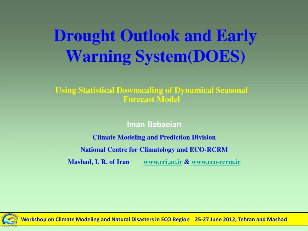
Drought Outlook and Early Warning System(DOES) ImanBabaeian Climate Modeling and Prediction Division National Centre for Climatology and ECO-RCRM Mashad, I. R. of Iran www.cri.ac.ir & www.eco-rcrm.ir Using Statistical Downscaling of Dynamical Seasonal Forecast Model
Contents • Review of Climate Modeling in ECO-RCRM • Time scale in predictions • Why seasonal prediction is possible? • Dynamical drought prediction • Seasonal forecast model • Data • Precipitation Forecast • SPI Forecast • Skill analysis • Conclusion
Review of Climate Modeling in ECO-RCRM • Short-term Weather Prediction Using WRF and MM5, • Regional Climate Modeling Using RegCM • Climate Change Modeling • Seasonal Forecast and Drought Early Warning
Regional Climate Modeling Using RegCM Humidity Advection From Pakistan • Source of humidity and summer rain fall of SE Iran is Pakistan, • Kuo convection scheme has skillful forecast over the region
Sensitivity of Different Schemes and Centre domain to RegCM precipitation • Skill of precipitation is increased when moving the centre • domain to the dominant synoptic pattern • In the northern regions and non-convective area, skil of • precipitation forecast is increased when using Grell schemes
Tele-connection modeling of the pressure patterns and precipitation H H L L Winter precipitation Decile-1991 Winter precipitation Decile-1996
L H Winter 2000 Winter 2000
Yearly runoff (above) and snowfallchange (bellow) over Caspian region, 2071-2100, PRECIS A2 (right) and B2 (left)
Precipitation Threshold to return period of 5 to 15 years during observation and 2010 to 2039
Time scale in predictions • Now-casting: Observation, Satellite, Radar ~ less 6 hours • Short-range forecasting: NWP models including WRF, MM5, . . . ~ less that 15 days-Dynamical downscaling • Seasonal forecasting: Climate models such as RegCM4, NCEP-RSM, . . . ~ 3 to 9 months
Inter-annual forecasting: TCC and Hadley Centre ~ 1 – 5 years, - Only uses SST boundary condition data - The most skillful area is tropical region which is covered by oceans • Decadal forecasting: Uses thescenarios prepared by IPCC,PRECIS is the famous model in this categor. . . ~ 10-100 years
Why seasonal forecast is possible? Surface temperature of the global oceans can influence weather patterns, These influences are not easily noticed in day-to-day weather events but become evident in long-term weather averages-It is good for seasonal forecasts, The slow fluctuations of sea-surface temperature (SST) can be predicted up to about 6 months ahead, The links between SST and weather can be represented in computer models of the atmosphere and ocean,
The strongest links between SST patterns and seasonal weather trends are found in tropical regions, The best known links are those associated with the El Niño phenomenon, The two key characteristics of seasonal forecasts are: -forecasts are for conditions averaged over three-month (seasonal) periods. -forecasts are stated in terms of probability.
Dynamical drought forecast A Seasonal Forecast System (NCEP-CFS, MRI-CGCM3) Downscaling of Model Precipitation Downscaling methods SPI Prediction Skill analysis
Some reference for this work A dynamically based SPI prediction has been developed over United State using NCEP-CFS modelbyYoon et. al. (2011), Their method was gridded instead of station scale, The skill was regionally and seasonally dependent, Luo et. Al. (2008) also worked on dynamically prediction of drought, They found that using multi-model methods is more skillful than one model of deterministic forecast.
Luo et. al. (2008) dynamically based Drought prediction over United State using NCEP-CFS model and percentage of soil moisture deficit,
Atmospheric Model • AGCM is spectral, developed based on JMA operational Numerical Weather Prediction (NWM),
Land Hydrology • Parameterization of ground hydrology is based on the Simple Biosphere(SiB) model that treat the effect of vegetation, • The model has three soil layers with different field capacity for each vegetation type, • Flow rate is set to move all the water storage in a grid box to next downstream grid in one time step, • When Snow cover exceeded than 10m equivalent water in Antarctica & Greenland, it discharges in the ocean, • Inland waters (Caspian & Aral Sea, Balkhash, Chad and Eyre Lake) are considered as terminal grid boxes with a drainage basin unconnected to ocean,
Storage of inland: water changes calculates by balance between river discharge and precipitation and evaporation over the water area, • Water temperature is predicted by the heat budget at the water surface, assuming 50m thick slab,
Ocean Model • The oceanic component is a Bryan-Cox type Ocean General Circulation Model (OGCM), • Horizontal spacing is 2.5 degree in longitude and 2 degree in latitude pole-ward of 12 degree, • Near the equator, between 4S to 4N, the meridional grid spacing is set 0.5 degree in order to provide good resolution equatorial oceanic waves, • Grid spacing gradually increases from 0.5 to 2 degree for latitudes of 4 to 12 degree, • Model has 23 layer in depth with 5.2m thickness, with 2 more layer for upper thermo-cline aiming aiming at a better representation of oceanic waves, • The deepest bottom is set to 5000m,
Denmark straight is made deeper and broader than real topography to represent sub-grid scale overflow of Nordic Sea aiming at improvement of thermo-cline circulation in North Atlantic, • Horizontal viscosity is and vertical viscosity coefficient is • Horizontal and vertical diffusivity of MRI-CGCM1 were 2.5 and 5 times larger than MRI-CGCM2 leading to sharper oceanic front because of high temperature gradient and stronger oceanic circulation and meridional overturning, • Solar radiation penetrating seawater is absorbed with e-folding of 10m-depth.
Sea Ice Model • The Sea Ice model is on the basis of Mellor and Kantha (1989), • The freezing and (melting) rate of sea ice is calculated with balance of heat and freshwater at the sea ice bottom, • Compactness is calculated using empirical constants, • The sea ice is advected by the empirical constant of 1/3,
Coupling Scheme • The atmosphere and the ocean interact with each other by exchanging fluxes of heat, freshwater and momentum at the sea surface, • Fluxes are exchanged every 24 hours in the model, • The AGCM integrates every 24hours fluxes at the sea surface. These fluxes are transferred to the OGCM grid. The OGCM is then time integrated for 24 hours, and resulting SST, sea ice compactness and thickness and surface wind for updating the lower boundary for the AGCM. These procedures are repeated.
Precipitation Forecast
Data • Two kind of data are used in this research, • They are: • Observed monthly station precipitation over 71 synoptic station of Iran • Period of data 1981-2007 • Modeled gridded data from MRI-CGCM3 from JMA • Period of gridded re-forecast data were 1981-2007
Observed data Caspian Sea A- Monthly precipitation over 71 synoptic station of Iran B- Period 1981-2007 Persian Gulf
Model Data (two series of data are used) A- 20 averaged gridded data B- 6 gridded data including: Prcp, SLP, T850, T-surf and H500 over station grid
Scores used to evaluate the skill of forecasts • Mean Square Error of Forecasts • Mean Square Error of Climatology • Mean Square Skill Score • Categorical (Percentage) Score Skill • Mean Bias Error • Relative Error
Downscaling Flowchart • MRI-CGCM3 • (26 model variables) • Observed Prcp. • (1 station variable) Computing partial correlations Select 3 best correlated model variables • Precipitation downscaling • (using multiple regression model)
Computing partial correlation Using JMP software
Multiple regression model to downscale / post processing the MRI-CGCM3 precipitation output
Skill of downscaling/post processing in February precipitation forecast Mashad - Feb. Precipitation(mm)