Download

1 / 24
240 likes | 401 Views
Temporal Analysis of Forest Cover Using a Hidden Markov Model. Arnt-Børre Salberg and Øivind Due Trier Norwegian Computing Center Oslo, Norway. IGARSS 2011, July 27. Outline. Motivation Hidden Markov model Concept Class sequence estimation

E N D
Temporal Analysis of Forest Cover Using a Hidden Markov Model Arnt-Børre Salberg and Øivind Due Trier Norwegian Computing Center Oslo, Norway IGARSS 2011, July 27
Outline • Motivation • Hidden Markov model • Concept • Class sequence estimation • Transition probabilities, clouds, and atmosphere • Application: Tropical forest monitoring • Conclusion
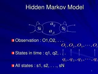
Introduction • Time-series of images needed in order to detect changes of the spatial forest cover • Time-series analysis requires methodology that • handles the natural variability between in images • overcome problems with cloud cover in optical images (and missing data in Landsat-7) • handles atmospheric disturbances • does not propagate errors from one time instant to the next
Introduction: Change detection • Naive • Simply create forest cover maps from two years, and compare • Errors in both maps are added. Not a good idea! • Time series analysis • Model what is going on by using all available images from the two years (and before, between, and after)
Hidden Markov Model (HMM) • HMM used to model each location on ground as being in one of the following classes: w = {forest, sparse forest, grass, soil} • Markov property: P(wt|wt-1,…,w1) = P(wt|wt-1)
Hidden Markov Model (HMM) • Bayes rule for Markov models • P(wt|wt-1) : class transition probability P(3|1) P(1|1) P(2|1) class 1 class 2 class 3
Class sequence estimation • Two popular methods for finding the class sequence W • Most likely class sequence • Minimum probability of class error
Most likely class sequence (MLCS) • Finds the class sequence that maximizes the likelihood →maximum likelihood estimate • The optimal sequence is efficiently found using the Viterbi-algorithm
Viterbi algorithm Forest Forest Sparse forest Sparse forest Grass Grass Soil Soil Most probable sequence of previous states for each state at time t Possible states at time t Possible states at time t+1 The probability of observing the actual observation, given that the state is k The probability of jumping from state c to state k (this is dependent on the time interval) The best sequence ending at state c, given the observations x1, …, xt
Minimum probability of class error • If we are interested in obtaining a minimum probability of error class estimate (at time instant t), the MLCS method is not optimal, but the maximum a posteriori (MAP) estimate is • The MAP estimate at time instant t • wt found using the forward-backward algorithm
Class transition probabilities • Landsat: Minimum time interval between two subsequent acquisitions is 16 days • Let P0(wt=m|wt=m’) = P0(m|m’) denote the class transition probability corresponding to 16 days • Class transition probability for any 16·Dt interval …in matrix form
Clouds • Clouds prevent us from observing the Earth’s surface • Clouds may be handled using two different strategies • Cloud screening and masking of cloud-contaminated pixels as missing observations • Include a cloud class in the HMM modeling framework …in this work we only consider strategy 1. • Cloud screening performed using a SVM
Data distributions, class transition probabilities, co-registration • Landsat image data (band 1-5,7) modeled using class dependent multivariate Gaussian distributions • Mean vector and covariance matrix estimated from training data • Class transition probabilities assumed fixed • May be estimated from the data (e.g. Baum-Welch) • Precise co-registration needed
Atmospheric disturbance Top of the atmosphere reflectance Atmosphere Ground surface reflectance • We apply a re-training methodology for handling image data variations (IGARSS’11, MO4.T05) • LEDAPS calibration (surface reflectance) will be investigated
Landsat 5 TM images (166/63)Amani, Tanzania 1985-03-09 1986-06-16 1986-08-19 1986-10-06 1987-08-06 1995-02-01 1995-02-17 1995-05-24 2008-06-12 2009-07-01 2009-11-06 2009-11-22 2009-12-08 2010-02-10
Results - Forest cover maps Forest Sparse forest Soil Grass Worldview-2 2010-03-04 1986-06-16 1995-02-17 2010-02-10
Results - Forest cover change Clouded observation 1986-06-16 1986-08-19 1986-10-06 1995-02-01 1995-02-17 Clouded observation Clouded observation 2009-07-01 2009-11-22 2009-12-08 2010-02-10 WV2 2010-03-25
Landsat 5 TM images (227-062)Santarém, Brazil 1988-09-04 1989-08-22 1992-07-29 1993-05-29 1995-06-04 1996-07-08 2004-08-31 2005-07-01 2005-07-17 2006-08-05 2007-06-21 2008-06-23 2008-09-11 2009-07-12 2009-07-28
Results - Forest cover mapsSantarém, Brazil 1986-07-29 1997-07-27 2008-06-23 2007-06-23
Results - Forest cover change mapsSantarém, Brazil 1986-07-29 1997-07-27 2008-06-23 2007-06-23
Multsensor possibilities • Multitemporal observations from other sensors (e.g., radar) may naturally be modeled in the hidden Markov model • Only the sensor data distributions are needed, e.g. • The multisensor images need to be geocoded to the same grid
Temporal forest cover sequence • Multisensor Hidden Markov model TIME wt-2 wt-1 wt wt+1 CLASSES yt-2 yt-1 yt yt yt+1 OBSERVATIONS Optical Optical Optical SAR Optical SAR
Conclusions • Time series analysis of each pixel based on a hidden Markov model • Finds the most likely sequence of land cover classes • Change detection based on classified sequence • Does not propagate errors since the whole sequence is classified simultaneously. • Regularized by the transition probabilities. • Handles cloud contaminated images • Multisensor possibilities
Acknowledgements The experiment presented here was supported by a research grant from the Norwegian Space Centre.