Download
1 / 14
140 likes | 246 Views
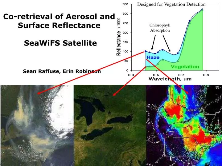
Designed for Vegetation Detection. Chlorophyll Absorption. Co-retrieval of Aerosol and Surface Reflectance SeaWiFS Satellite. Sean Raffuse, Erin Robinson. Co-Retrieval of Surface and Aerosol Properties Apparent Surface Reflectance, R.

E N D
Designed for Vegetation Detection Chlorophyll Absorption Co-retrieval of Aerosol and Surface Reflectance SeaWiFS Satellite Sean Raffuse, Erin Robinson
Co-Retrieval of Surface and Aerosol PropertiesApparent Surface Reflectance, R • The surface reflectance R0 objects viewed from space is modified by aerosol scattering and absorption. • The apparent reflectance, R, is: R = (R0 + Ra) Ta Apparent Reflectance R may be smaller or larger then R0, depending on aerosol reflectance and filtering. Surface Reflectance The surface reflectance R0is an inherent characteristic of the surface Aerosol Reflectance Aerosol scattering acts as reflectance, Ra adding ‘airlight’ to the surface reflectance Aer. Transmittance Both R0 and Ra are attenuated by aerosol extinction Ta which act as a filter Aerosol as Filter: Ta = e-t Aerosol as Reflector: Ra = (e-t – 1) P R = (R0 + (e-t – 1) P) e-t
Co-Retrieval: Seasonal Surface Reflectance, Eastern US April 29, 2000, Day 120 July 18, 2000, Day 200 October 16, 2000, Day 290
Kansas Agricultural Smoke, April 12, 2003 Organics 35 ug/m3 max Fire Pixels PM25 Mass, FRM 65 ug/m3 max Ag Fires SeaWiFS, Refl SeaWiFS, AOT Col AOT Blue
Kansas Smoke April 12, 2003 April 10, 2003
Kansas Smoke Emission Estimation April 11, 2003 Assuming Mass Extinction Efficiency: 5 m2/g April 10: 1240 T/d April 11: 87 T/day Monte Carlo Diagnostic Local Model Emission Estimate Fire Pixels Surface Observations
Fire Model Land Vegetation Emission Model Satellite-Surface-Model Data IntegrationSmoke Emission Estimation Continuous Smoke Emissions Assimilated Smoke Emission for Available Data Local Smoke Simulation Model e..g. MM5 winds, plume model Assimilated Fire Location Assimilated Smoke Pattern Fire Location Satellite Smoke Surface Smoke Fire Pixel, Field Obs AOT Aer. Retrieval Visibility, AIRNOW
Satellite Aerosol Optical Thickness ClimatologySeaWiFS Satellite, Summer 2000 - 2004 20 Percentile 60 Percentile Smoke Sources 98 Percentile 90 Percentile 98 Percentile
Summer AOT 60 Percentile 2000-2004 SeaWiFS AOT, 1 km Resolution Birmingham Atlanta Mountain – Low AOT Valley – High AOT Cloud Contamination?
Temporal Signal Decomposition and Event Detection EUS Daily Average 50%-ile, 30 day 50%-ile smoothing • Daily median & average over a region • Temporal smoothed by a 30 day Event : Deviation > x*percentile Deviation from %-ile Average 3. Event is the deviation of daily value from the smooth median (event – red; noise blue) Mean Seasonal Conc. Median Median Seasonal Conc.
Causes of Temporal Variation by Region The temporal signal variation is decomposable into seasonal, meteorological noise and events. Statistically: V2Total =V2Season +V2MetNoise +V2Event Northeast exhibits the largest coeff. variation (56%); seasonal, noise and events each at 30% Southeast is the least variable region (35%), with virtually no contribution from events Southwest, Northwest, S. Cal. and Great Lakes/Plains show 40-50% coeff. variation mostly, due to seasonal and meteorological noise. Interestingly, the noise is about 30% in all regions, while the events vary much more, 5-30%
Origin of Fine Dust Events over the US Gobi dust in spring Sahara in summer Fine Dust Events, 1992-2003 ug/m3 Fine dust events over the US are mainly from intercontinental transport