
Statistics for Water Science
E N D
Presentation Transcript
Statistics for Water Science Module 17.1: Descriptive Statistics
Module 17: Statistics • Statistics • A branch of mathematics dealing with the collection, analysis, interpretation and presentation of masses of numerical data • Descriptive Statistics (Lecture 17.1) • Basic description of a variable • Exploratory Data Analysis (Lecture 17.2) • Techniques for understanding data • Hypothesis Testing (Lecture 17.3) • Asks the question – is X different from Y?
Simple graphical representations of data Describe basic characteristics of a population of numbers Central Tendency or “Middleness” Means, medians and others Variance or “spread” of data Standard Deviation The range of data Min, Max and Percentiles Descriptive statistics
Precision: Tendency to have values closely clustered around the mean Accuracy: Tendency of an estimator to predict the value it was intended to estimate Bias: A systematic error in prediction Adapted from Ratti and Garton (1994) Precision, accuracy and bias
Unbiased Biased The yellow curling rocks represent means from repeated samples Green dots are the mean value Spread is analogous to the standard error Not Precise Precise Accurate Not Accurate
Between 1998 and 2002, the Ice Lake RUSS unit collected 2120 temperatures readings at depths of 1-4 m What is the average June temperature? Finding the middle:The arithmetic mean
39179.3 2120 = 18.48 C Finding the middle:The arithmetic mean • Not too hard - Add’em up, divide by n Sum of temperatures = 39179.3
Expressing variability: Standard deviation (SD) • Note that there is ‘scatter’ around the mean • The Standard Deviation quantifies how wide or narrow this scatter is: • For this data set, the SD is 2.34 C • Mean and SD are often combined: • 18.48 +/- 2.34
n = 3097 Comparing data sets • Let’s consider a second data set, shown in blue. This is the mean seasonal temperature in the lower reaches of the lake (8-13 m)
Comparing data sets • Two things to note: • It’s a lot colder at the bottom of the lake! • The temperatures are much less variable – why?
Means and standard deviations for epilimnetic and hypolimnetic temperatures
Standard deviation: Fun facts • The SD is always in the same units as the mean • Roughly 68% of the values are included in +/- 1 SD of the mean, 95% within +/- 2 SD • If the SD is larger than the mean (e.g. 20 +/- 24), your data is pretty flaky • Definition of flaky – the data are so widely scattered that the mean is, well, meaningless. • In this case, use some other measure of middleness, such as the geometric mean or median
What about data that are not well behaved? Fecal coliform counts are often used by management agencies as an indicator of water quality For non-contact water recreation (boating and fishing), Colorado Public Health state that fecal coliform count shall not exceed 2000 fecal coliforms per 100 mL (based on geometric mean of representative samples) Using geometric means: Fecal coliform example
12000 Boulder Creek Longitudinal Fecal Coliform Profiles for July, 2000 The problem • Fecal coliform counts can range over several orders of magnitude. • For such data, the geometric mean is a more appropriate indicator of central tendency.
4 Geometric mean = 160 * 700 * 60 * 12000 The geometric mean • Multiply ’em together, take the nth root • To be honest, this is a pain without a good calculator, but there’s a shortcut…
The geometric mean: The easy way • Take the logarithm of each data point (easy)
The geometric mean • Take the logarithm of each data point (easy) • Average the log values (easier)
The geometric mean • Take the logarithm of each data point (easy) • Average the log values (easier) • Calculate the antilog (sounds hard, is easy) • Antilog = 10^2.88 = 764.1 • The geometric mean is 764.1 cells/ 100 ml • Lower than the state regulatory standard of 2000 cells/ 100 ml
Fun facts about geometric means • The geometric mean is always less then the arithmetic mean. • The ‘shortcut’ calculation works with either natural logs or base 10 logs. • The geometric mean tends to dampen the effect of very low or very high values, and is useful when values range from 10-10,000 over a given period. • Excel has a GEOMEAN function. Life is good. • Use of the geometric mean is a standard for most wastewater discharge and beach monitoring programs: • Beach standards are typically 200 counts/100 ml.
When to use medians: Stream turbidity levels • Background: • Turbidity in streams makes the water appear cloudy (muddy), mostly from suspended sediments. It’s bad for fish, their eggs and their food (bugs) – particularly cold water species such as brook trout. • Minnesota Water Pollution Rules set a Chronic Standard of 10 NTU - the highest level to which these organisms can be exposed indefinitely without causing chronic toxicity (see Notes for reference website). • Tischer Creek is a trout stream in Duluth, MN with a nearly continuous turbidity record in summer/fall 2002. Let’s look at a 30 day period in midsummer and decide what the level of exposure was for the fish.
Medians: the middlemost value • Prevents being mislead by a few very small or very large values • Consider salaries within a hypothetical company • Which is the more appropriate measure of a typical salary? • Mean $104,000 • Median $24,000
Medians: a real world exampleTischer Creek: July 13 - Aug 12, 2002
Frequency Distribution: Jul 13- Aug 12Tischer Creek – Summer 2002 Note that these data are highly skewed, with >80% of the values in the 20-40 NTU range There is one value of 1017 NTU, no valid reason to delete it.
Stream Data Visualization • Tischer Creek –Summer 2002 Storm Period
Means vs Medians: Which represent the data better? • The mean of 13 NTU for the 30 day period suggests that the chronic toxicity standard was violated • The standard deviation of the mean was high (48 NTUs) relative to the mean and so the coefficient of variation was a whopping 369%: CV = (48/13)*100 • Although the range was high, from 0 to 1017 NTU, “most of the time” the stream ran clear with values <<10 . The mode (most common value) was in fact = 0 • The median value was 1.0 NTU and perhaps best characterizes the state of turbidity in the stream and the level of exposure of the fish (the 50th percentile). • Determining chronic exposure values for “flashy” data is not trivial
Excel functions for descriptive statistics: Format - @statistic(datarange)
Upcoming: How can we tell if two populations of numbers are different?