Efficient MCMC for cosmological parameters

1. Efficient MCMC for cosmological parameters Antony Lewis Institute of Astronomy, Cambridge http://cosmologist.info/ collaborator: Sarah Bridle CosmoMC: http://cosmologist.info/cosmomc Lewis, Bridle:astro-ph/0205436 http://cosmologist.info/notes/cosmomc.ps.gz

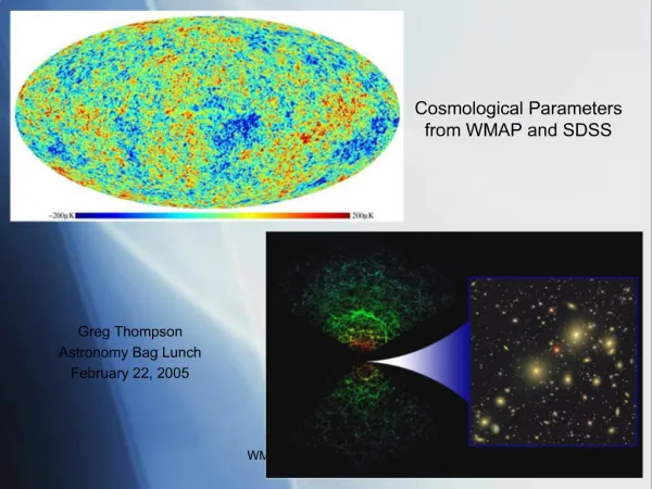
2. Introduction CMB PolarizationBaryon oscillations Weak lensing Galaxy power spectrum Cluster gas fraction Lyman alpha etc… + + Priors WMAP Science Team Cosmological parameters

3. Bayesian parameter estimation • Can compute P( {ө} | data) using e.g. assumption of Gaussianity of CMB field and priors on parameters • Often want marginalized constraints. e.g. • BUT: Large n-integrals very hard to compute! • If we instead sample from P( {ө} | data) then it is easy: Generate samples from P

4. old CMB data alonecolor = optical depth Samples in6D parameterspace

5. Markov Chain Monte Carlo sampling • Move in parameter space with transition probability: Chain distribution converges to P if all points can be reached (ergodic) andT leaves the distribution invariant for all θ’ • Detailed balance is a sufficient condition: Metropolis-Hastings method: for (nearly) arbitrary proposal function q and Simplest if q chosen to be symmetric

6. If proposed position has higher probability: always move P(x) 0 x1 x2

7. If proposed position has lower probability: move to x2 with probability P(x2)/P(x1) otherwise take another sample at x1 P(x) P(x1) ? P(x2) 0 x2 x1

8. Procedure:- Chose priors and parameterization - Chose a proposal distribution- Start chain in some random position (or several in different starting positions)- Iterate large sequence of chain steps storing chain positions (correlated samples)- Remove ‘some’ samples from the beginning (‘burn in’) - Optionally thin the samples- Check for convergence - Estimate desired quantities from samples (or just publish list of samples)

9. Potential Problems: - Proposal width low or directions bad: slow sqrt(N) random walk through space - Proposal width too large: low probability of proposing similar likelihood, low acceptance rate- Proposal distribution must be able to reach all points in parameter space Can never cross gap!

10. Assessing performance and convergence From single chain: • - Autocorrelation length • Raftery and Lewis • Chain splitting variances From multiple chains (e.g. MPI): Gelman-Rubin (last half chains): - variance of means - diagonalized variance of means - diagonalized variance of limits All necessary but not sufficient!

11. Which proposal distribution? Possible approaches: • Use many different proposals, try to be as robust as possible – ‘black box’:- e.g. BayeSyshttp://www.inference.phy.cam.ac.uk/bayesys/ • - Unnecessarily slow for ‘simple’ systems. - Less likely to give wrong answers.- Versatile (but work to integrate with cosmology codes). • Use physical knowledge to make distribution ‘simple’ – use simple fast method: • e.g. CosmoMC- Fast as long as assumptions are met. - More likely to give wrong answers; need e.g. close to unimodal distributions.- Less versatile- Optimized to use multi-processors efficiently; integrated CAMB • Either of above, but also try to calculate ‘Evidence’: - e.g. BayeSys, Nested Sampling (CosmoMC plug-in), fast method + thermodynamic integration, etc… Essentially no method is guaranteed to give correct answers in reasonable time!

12. Proposal distribution: Use knowledge to change to physical parameters • E.g. peak position ~ • sound horizon • -------------------------------- • angular diameter distance • use this as variable • if non-linear transformation beware of priors (Jacobian) Kosowsky et al. astro-ph/0206014

13. Proposal distribution: changing variables, transform to near-isotropic Gaussian Linear Transformation No change in priors Equivalent to proposing alongeigenvector directions Easily done automatically from estimate of covariance matrix e.g.

14. Proposal distribution: dynamically adjusting parameters Beware of non-Markovian updates…OK methods: • Do short run, estimate covariance, change parameters, do final run-Make periodic updates, but discard all samples before the final update • Periodically update covariance, but use constant fraction of all previous samples; covariance will convergence, hence asymptotically Markovian BAD methods (sample from wrong distribution, e.g. astro-ph/0307219): - Estimate local covariance and use for proposal distribution - Dynamically adjust proposal width based on local acceptance rate - Propose change to some parameters then adjust other parameters to find good fit, then take new point as final proposal ?? The onus is on you to prove any new method leaves the target distribution invariant!

15. Symmetric Metropolis proposal distributions - Most common choice is a n-D Gaussian (n may be a sub-space dimension) - in 2D - Scale with to n get same acceptance rate in any dimension - In general corresponds to choosing random direction, and moving normalizeddistance r in that direction with probability ‘Best’ scaling is r→r / 2.4 if posterior is GaussianDunkley et al astro-ph/0405462 Q: Is this really best, or just shortest autocorrelation length??

16. Is using a large-n Gaussian proposal a good idea?e.g. consider Pn(r) as a proposal in 1D – be careful how you assess performance! Higher n, shorter correlation length, worse Raftery & Lewis Definitely not in 1D… maybe not in general

17. Want robust to inaccurate size estimates: broaden tail, make non-zero at zero: e.g. mixture with exponential 1/3 exponential, n=2, 5 (n=2 used by CosmoMC) +cycling

18. Fast and Slow Parameters • Calculating theoretical CMB and P(k) transfer functions is slow (~ second) ‘Slow’ parameters: - Changing initial power spectrum is fast (~ millisecond) ‘Fast’ parameters: • Other nuisance parameters may also be fast (calibrations etc.), though often can be integrated numerically. • ‘Fast’ only as fast as the data likelihood code How do we use the fast/slow distinction efficiently?

19. Usual choice of proposal directions: Fast-slow optimizedchoice: Slow Fast

20. ‘Directional Gridding’ (Radford Neal) Slow Slow grid width chosen randomlyat start of eachgridding step: fullgridding step leavesdistribution invariant Fast Other methods: e.g. tempered transitions etc. may work for very fast parameters Variation of: Neal 1996; Statistics and Computing 6, 353 Neal 2005, math.ST/0502099 (Nested sampling??)

21. Choice of Priors e.g. parameterize reionization history in a set of bins of xe. What is your prior? P(τn) • Physically 0 < xe < 1- ‘Simple’ choice is uncorrelated uniform flat prior on optical depth from each bin: 1/τn 0 τn Lewis et al. 2006, in prep

22. What does this mean for our prior on the total optical depth? Exact result is piecewise polynomial Large N Total optical depth prior ~ Gaussian (strongly peaked away from zero).Low optical depth is a priori very unlikely - is this really what you meant??

23. If you don’t have very good data worth thinking carefully about your prior! Another example: reconstructing primordial power spectrum in n bins Bridle et al. astro-ph/0302306 or ? with flat uncorrelated priors on bins? Differ by an effective prior on optical depth ! Also, do we really mean to allow arbitrarily wiggly initial power spectra? One sensible solution: Gaussian process prior (imposes smoothness) - result then converges for large n

24. Conclusions • MCMC is a powerful method, but should be used with care • Judicious choice of parameters and proposal distribution greatly improves performance • Can exploit difference between fast and slow parameters • Worth thinking carefully about the prior • Do not run CosmoMC blindly with flat priors on arbitrary new parameters

25. Random directions? Don’t really want to head back in same direction… • Chose random orientation of orthogonalized basis vectors • Cycle through directions- Periodically chose new random orientation Helps in low dimensions Also good for slice sampling (sampling_method=2,3) (Neal: physics/0009028) mixture only

26. Using fast-slow basis: - Less efficient per step because basis not optimal- Can compensate by doing more ‘fast’ transitions at near-zero cost- Ideally halves the number of ‘slow’ calculations Can be generalized to n-dimensions: - make several proposals in fast subspace - make proposals in best slow eigendirections - save lots of time if many fast parameters This is CosmoMC default