Download
1 / 45
450 likes | 599 Views
Application of the MCMC Method for the Calibration of DSMC Parameters. James S. Strand and David B. Goldstein The University of Texas at Austin. Sponsored by the Department of Energy through the PSAAP Program. Predictive Engineering and Computational Sciences. Introduction – DSMC Parameters.

E N D
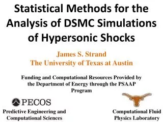
Application of the MCMC Method for the Calibration of DSMC Parameters James S. Strand and David B. Goldstein The University of Texas at Austin Sponsored by the Department of Energy through the PSAAP Program Predictive Engineering and Computational Sciences
Introduction – DSMC Parameters • Direct Simulation Monte Carlo (DSMC) is a valuable method for the simulation of rarefied gas flows. • The DSMC model includes many parameters related to gas dynamics at the molecular level, such as: • Elastic collision cross-sections • Vibrational and rotational excitation cross-sections • Reaction cross-sections • Sticking coefficients and catalytic efficiencies for gas-surface interactions. • …etc.
Introduction – DSMC Parameters • In many cases the precise values of some of these parameters are not known. • Parameter values often cannot be directly measured, instead they must be inferred from experimental results. • By necessity, parameters must often be used in regimes far from where their values were determined. • More precise values for important parameters would lead to better simulation of the physics, and thus to better predictive capability for the DSMC method.
MCMC Method - Overview • Markov Chain Monte Carlo (MCMC) is a method which solves the statistical inverse problem in order to calibrate parameters with respect to a set or sets of experimental data.
MCMC Method Establish boundaries for parameter space Candidate Accepted Candidate Rejected Accept or reject candidate position based on a random number draw Select initial position Current position remains unchanged. Candidate position becomes current position Run simulation at current position Probcandidate < Probcurrent Run simulation for candidate position parameters, and calculate probability Calculate probability for current position Select new candidate position Probcandidate > Probcurrent Candidate position is accepted, and becomes the current chain position Candidate automatically accepted
MCMC Method - Steps • Simple example illustrates the MCMC method.
1D Shock Simulation • Base flow is a 1D, unsteady shock, moving through the computational domain. • A set of sample cells moves with the shock. These sample cells continuously collect data on the shock profile. • This method allows for a smooth solution in an unsteady flow without the computational cost of ensemble averaging or using excessively large numbers of particles. • No prior knowledge of the post-shock conditions is required.
1D Shock Simulation – Measure of Error Alsmeyer’s Data Sample DSMC Results
Parallelization • DSMC: • DSMC code is MPI parallel, with dynamic load rebalancing periodically during each run. • Allows very fast simulation of small problems. • Super-linear speed-up due to better cache use. • Simulations which took 20 minutes on 1 processor take less than 20 seconds on 64 processors. • Faster DSMC simulations allow for much longer chains to be run in a practical amount of time. • MCMC: • Any given chain must be run in sequence. • MCMC method can be parallelized by running multiple chains simultaneously.
MCMC Parallelism All Processors
MCMC Parallelism All Processors Group 1 Group 3 Group 4 Group 6 Group 5 Group 2
MCMC Parallelism All Processors Group 1 Group 3 Group 4 Group 6 Group 5 Group 2 MCMC Chain 1 MCMC Chain 3 MCMC Chain 2
MCMC Parallelism All Processors Group 1 Group 3 Group 4 Group 6 Group 5 Group 2 MCMC Chain 1 MCMC Chain 3 MCMC Chain 2 MCMC Chain 5 MCMC Chain 4 MCMC Chain 6
MCMC Parallelism All Processors Group 1 Group 3 Group 4 Group 6 Group 5 Group 2 MCMC Chain 1 MCMC Chain 3 MCMC Chain 2 MCMC Chain 5 MCMC Chain 4 MCMC Chain 6 MCMC Chain 7 MCMC Chain 8
MCMC Parallelism All Processors Group 1 Group 3 Group 4 Group 6 Group 5 Group 2 MCMC Chain 1 MCMC Chain 3 MCMC Chain 2 Group 2 MCMC Chain 5 MCMC Chain 4 MCMC Chain 6 Group 1 MCMC Chain 7 MCMC Chain 8
MCMC Parallelism All Processors Group 1 Group 3 Group 4 Group 6 Group 5 Group 2 MCMC Chain 1 MCMC Chain 3 MCMC Chain 2 MCMC Chain 5 MCMC Chain 4 MCMC Chain 6 MCMC Chain 6 MCMC Chain 7 MCMC Chain 8
MCMC Parallelism All Processors Group 1 Group 3 Group 4 Group 6 Group 5 Group 2 MCMC Chain 1 MCMC Chain 3 MCMC Chain 2 Group 1 MCMC Chain 5 MCMC Chain 4 MCMC Chain 6 Group 3 MCMC Chain 6 MCMC Chain 7 MCMC Chain 8 Group 4
MCMC Parallelism All Processors Group 1 Group 3 Group 4 Group 6 Group 5 Group 2 MCMC Chain 1 MCMC Chain 3 MCMC Chain 2 MCMC Chain 5 MCMC Chain 4 MCMC Chain 6 MCMC Chain 6 MCMC Chain 7 MCMC Chain 8
First Calibration - Hard-Sphere Model • Parameter to be calibrated is dHS, the hard-sphere diameter for argon. Normalized density profile for a Mach 3.38 shock in argon from Alsmeyer (1976) used for calibration. • Uniform sampling method used to explore the parameter space. • Metropolis-Hastings MCMC algorithm used to solve inverse problem.
Second Calibration - VHS Model • Parameters to be calibrated are dref and ω, the reference diameter and the temperature-viscosity exponent for argon. Normalized density profile for a Mach 3.38 shock in argon from Alsmeyer (1976) once again used for calibration.
Second Calibration - VHS Model • For two parameter case, uniform sampling could still be used to explore parameter space. Simulation was run for each set of parameters on a 100×100 grid in parameter space, and a probability was calculated for each based on the error and the likelihood equation. A total of 10,000 shocks were simulated for the uniform sample.
Second Calibration - VHS Model • Band structure seen here indicates that this single dataset does not provide enough information to allow unique values to be determined for both dref and ω.
Second Calibration - VHS Model • MCMC calibration was also performed for this case. 64 chains were run, each with 4000 positions, for a total of 256,000 shocks. Full MCMC run took 20 hours on 4096 processors. • MCMC is overkill for this two-parameter system.
Second Calibration - VHS Model • Individual MCMC chains also show the band structure.
Second Calibration - VHS Model • The same band structure is seen in a scatterplot of MCMC chain positions and in a contour plot showing the number of MCMC chain positions in any given region.
Second Calibration - VHS Model • We can also see the band structure by directly viewing the probabilities at each MCMC chain position.
Conclusions/Future Work • MCMC successfully reproduces the results from a brute-force uniform sampling technique for the calibration of the parameters for the hard-sphere and VHS methods. • The normalized density profile from a single shock is insufficient to uniquely calibrate both parameters of the VHS method. • Temperature and velocity distribution function data provide better calibration for the VHS parameters. • The addition of internal energy modes and chemistry will increase both the number of parameters and the volume of available calibration data.