Download

1 / 64
640 likes | 839 Views
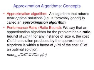
What should be taught in approximation algorithms courses? Guy Kortsarz, Rutgers Camden. Advanced issues presented in many lecture notes and books:. Coloring a 3- colorable graph using vectors. Paper by Karger , Motwani and Sudan . Things a student needs to know:

E N D
What should be taught in approximation algorithms courses?Guy Kortsarz, Rutgers Camden
Advanced issues presented in many lecture notes and books: • Coloring a 3-colorable graph using vectors. • Paper by Karger, Motwani and Sudan. • Things a student needs to know: Separation oracle for: A is PSD. Getting a random vector inRn. This is done by choosing the Normal distributionat every entry. Given unit vector v, v . ris normal distribution.
Things a student needs to know: • There is a choice of vectors vi for every i V so thatso that for every(i, j) E, vi · vj -1/2.
A student needs to know: • S={i | r · vi }, threshold method, by now standard. • Sum of two normal distributions also normal. • Two inequalities (non trivial) about the normal distribution. • The above can be used to find a large independent set. • Combined with the greedy algorithm gives about n1/4 ratio approximation algorithm.
Advanced methods are also required in the following topics often taught: • The seminal result of Jain. With the simplification of Nagarajan et. al. 2-ratio for Steiner Network. • The beautiful 3/2 ratio by Calinesco, Karloff and Rabani, for Multiway Cuts: geometric embeddings. • Facharoenphol, Rao and Talwar, optimal random tree embedding. With this can get O(log n)for undirected multicut.
How to teach sparsest cut? • Many still teach the embedding of a metric into L1, withO(log n)distortion. By Lineal, London, Rabinovich. • Advantage: relatively simple. • The huge challenge posed by the Arora, Rao and Vazirani result. Unweighted sparsest cutsqrt{log n} • Teach the difficult lemma? Very advance. Very difficult. • A proof appears in the book of Shmoys and Williamson.
Simpler topics? • I can not complain if it is TAUGHT! Of course not. Let me give a list of basic topics that always taught • Ratio3/2 for TSP, the simple approximation of 2 for min cost Steiner tree. • Set-Cover , simple approximation ratio. • Knapsack,PTAS. Bin packing, constant ratio. • Set-Coverage. BUT:only costs 1.
Knapsack Set-Coverage • The Set-Coverage problem is given a set system and a numberkselectk sets that cover as many elemnts as possible. • Knapsack version, not that known: • Each set has cost c(s) and there is a bound B on the maximum sum of costs, of sets we can choose. • Maximize number of elements covered.
Result due to Khuller , Moss and, Naor, 1997, IPL • The (1-1/e) ratio is possible. • In the usual algorithm & analysis (1-1/e) only follows if we can add the last set in the greedy choice. Thus, fails. • Because most times, adding the last set will give cost larger than B. • Trick: guess the 3 sets in OPTof least cost. Then apply greedy (don’t go over budget B).
Why do I know this paper? • I became aware of this result only several years after published. And only because I worked on Min Power Problems. No conference version! • This result seems absolutely basic to me. Why is it no taught? • Remark: Choosing one (least cost) element of OPT gives unbounded ratio. Choosing two sets of smallest cost gives ratio ½. Guessing the three sets of least cost and then greedy gives(1-1/e).
First general neglected topic • Important and not taught: Maximizing a submodular non-decreasing function under Matroid Constrains, ratio 1/2, Fischer, Nemhauser, Wolsey, 1977. • Improved in 2008(!) to best possible (1-1/e) by Vondrak in a brilliant paper.
First story: a submission I refereed • I got a paper to referee, and it was obvious that it is maximize Submodular function under Matroid constrains • If memory serves, the capacity 1, of the following Matroid: G(V,E), edge capacities, fix S V. T reaches S if every vertex in Tcan send one unit of flow toS. • The set of all T that reach S a special Matroid called Gammoid. Everything in this paper, known! • Asked Chekuri (everybody must have an oracle) what is the Matroid, and Chekuri answered. Paper erased.
Story 2: a worse outcome. • Problem. Input like Set-Cover but S= Si. • Required: choose at most one set of everySi and maximize the number of elements covered. • Paper gave ratio ½. This is maximizing submodular cover subject to partition Matroid. PLEASE!!! Do not try to check who the authors are. Not ethical. Unfair to authors, as well. • Nice applications, but was accepted and ratio not new.
Related to pipage rounding • Due to Ageev, Sviridenko. • Dependent rounding, is a generalization of Pipage rounding by Gandhi, Khuller, Parthasarathy, Srinivasan. • Say that we have an LP and a constraint xi=k. RR can not derive exact equality. • Pipage Rounding : instead of going to a larger set of solutions like IP to LP, we replace the objective function.
The principals of pipage rounding • We start with LP maximization with function L(X). • Define a non linear function F. • Show that the maximum of F is integral. • Show that integral points of F belong to the Polyhedra of L. Namely feasible for L as long as it is integral, and feasible for F.
The principals of pipage rounding • Then, show that F(Xint ) ≥L(X* )/, for > 1. • HereXint is the (integral) optimumof F and X*the optimum fractional solution for L • Because Xint is known to be feasible for L(x) due to its integrality, it is feasible for L and thus approximation.
Example: Max Coverage • Max j wi zi S.T element j belongs to set i xi≥zj set i xi=p xi and zj are integral In Set Coverage we bound the number of sets.
The function F • F(x)=j wi (1-element j belongs to set i(1-xi) ) • Definea function on a cycle. • As a function of . • The idea is to make plus and then minus over the cycle. • Make one entryonthe cycle smaller by and another larger by .
The function F • F(x)=j wi (1-element j belongs to set i(1-xj) ) • The idea is to make plus and then minus all over the cycle. • But to show convexity we make just one entryonthe cycle smaller by and another larger by . • The appears as 2 in this term.
The function F • As appears as 2 in this term, the second derivative is positive. • Thus F is convex. • Which means that the maximum is in the borders. • For example for x2 between -4 and 3. • The maximum is in the border -4.
Changing the two by two • Putting plus and minus alternating along a cycle make at least one entry integral. • Moreover, we can decompose a cycle into two matching and there are two ways to increase and decrease by . • One direction of the two makes the function not smaller. • This implies that the optimum of F is integral.
Thus the optimum of F is integral • Its not hard to see that on integral vectors F and L have the same value. • Another inequality that is quite hard to prove is that: 1-i=1 to k (1-xi)≥(1-(1-1/k)k)L(X) • This gives a slightly better than 1-1/e ratio if k is small.
Submodularity: related to very basic technique. • f is submodular if f(A)+f(B)f(AB)+f(AB) • Makes a lot of difference if non-decreasing or not. If not, in my opinion represent concave. • If non-decreasing, brings us to the next lost simple subject: Submodular cover problems. • Input: U and submodular non-decreasing function f and cost c(u) per item u. • Required: a set S of minimum cost so that f(S)=f(U).
Wolsey , 1982, did much better • Each iteration pick item u so that helpu(S)/c(u) is maximum. • The ratio is max{uU}ln f(u)+1. • Example: For Set-Coverln|s|+1,s largest set. • Example: Same for Set-Cover with hard capacities. A paper in 1991, and one in 2002, did this result again (second was 20 years after Wolsey). Special case after 20 years! But its worse, yet. • Wolsey did better than that. Natural LP unbounded ratio even for Set-Cover with hard capacities. • Wolsey found a fabulous LP of gap max{uU}ln f(u)+1.
More general: density • Not taught at all but just cited. Why? • Here is a formal way: • Universe U and a function f: 2UR+ • Each element in U has a cost c(u). • The function f not decreasing. • We want to find a minimum cost W so that f(W)=f(U). • We usually say, S U, c(S)=uS c(u) • But it works for an subadditive cost function
The density claim • Say that we already created a set S via a greedy algorithm. • Now say that at any iteration we are able to find some Z so that: (f(Z+S)-f(S))/c(Z)≥(f(U)-f(S))/(δ·opt) • Then the final set S has cost bounded by (δ ln(U)+1) opt
What does it mean? • Think for the moment of δ=1. • Say that the current set S has no intersection with the optimum. • Then if we add all of OPT to S we certainly get a feasible solution. • Then clearlyf(S+OPT)=f(U) • And • (f(S+OPT)-f(S))/c(Z)≥ (f(OPT)-f(S))/c(OPT) • =(f(U)-f(S))/f(OPT) • It means that we found a solution to add that has the samedensity as adding OPT.
Proof continued • f(U) - j≤ i-1 f(Sj)≥ 1. • We may assume that the cost of every set added is at most opt, therefore c(Sj ) ≤opt • Therefore it remains to bound: j≤ i-1 c(Zi) Let us concentrate on what happens before Si is added.
By the previous claims • 1 ≤ f(U)-f(Z1+Z2 +……Zi-1)≤ Πj≤ i-1(1-c(Zi)/δ·opt)· f(U) • 1/f(U) ≤ Πj≤ i-1(1-c(Zi)/δ·opt)· • Take ln and use ln(1+x) ≤ x: -ln( f(U))≤ i≤ j -c(Zi) )/δ·opt i≤ j c(Zi) ≤opt δ ln( f(U)) and so the ratio of (δ ln( f(U))+1) follows.
A paper of mine • Min c x subject to ABx b, with A positive entries and B flow matrix. Ratio logarithmic. • We got much more general results. The above I was sure then and sure now, KNOWN and presented as known. • Referees: Cite, or prove submodularity! We had to prove (referees did not agree its known!). • Example: gives log n for directed Source Location. Maybe first time stated but I considered it known. • This log n was proved at least 4 times since then.
Remarks • The bad thing about these 4 papers is not that did not know our paper (to be expected) but that they would think such a simple result is NOTKNOWN. • It is good to know the result of Wolsey: for example, used it recently (Hajiaghayi ,Khandekar,K , Nutov) to give a lower bound of about log 2 n for a problem in fashion: Capacitated NetworkDesign (Steiner network with capacities). First lower bound for hard capacities.
Dual fitting and a mistake we all make • 1992. GK to Noga Alon: • This (spanner) result bares similarities to the proof done by Lovats for set-cover. • Noga Alon (seems very unhappy, maybe angry): Give me a break! That is folklore. Lovats told me he wrote it so he would have something to cite....... • Everybody cites Lovats here. Its simply not true. • We don’t know the basics. Result known many years before 1975. • Should we cite folklore? Yes!
HOW to teach dual fitting for set cover, unweighted? • Let S be the collection of sets and Tthe elements. • The dual, costs 1: MaximizetT yt • Subject to: ts yt c(s)=1 • We define a dual: if the greedy chose a star of length i, each element in the set gets 1/i .2 .2 .2 .2 .2
The bound on the sum of elements of a given set 1/2 1/2 1 1/7 1/6 1/7 1/5 1/7 1/4 1/4 1/3 1/12 1/12 1/11 1/12 1/10 1/9 1/12 1/8 1/12
Primal Dual of GW • Goemans and Williamson gave a rather well known Primal-Dual algorithm. Always taught, and should be. • A question I asked quite several researchers and I don’t remember a correct response: Why reverse delete? • Why not Michael Jackson? • GW primal dual imitates recursion. • In LR reverse delete follows from recusrsion.
Local Ratio for covering problems • Give weights to items so that every minimal. solution is a approximation. Reduce items costs by weights chosen. • Elements of cost 0 enter the solution. • Make minimal. • Recurse. • No need for reverse delete. Recursion implies it. • Simpler for Steiner Network in my opinion.
Local Ratio • Without it I don’t think we could find a ratio 2 for Vertex feedback set. • A recent result of K, Langberg, Nutov. Minor result (main results are different) but solves an open problem of a very smart person: Krivelevich. • Covering triangles, gap2for LP (polynomial). • Open problem: tight? • Not only we showed tight family but showed as hard as approximatingVC.Used LR in proof.
Group Steiner problem on trees • Group Steiner problem on trees. • Input : An undirected weighted rooted by r tree T = (V; E) and subsets S1,……,Sp V. • Goal: Find a tree in G that connects at least one vertex from each Si to r. • The Garg,Konjevod and Ravi proof while quite simple can be much much further simplified. In both proofs: O(log n· log p) ratio. • The easier (unpublished) proof is by Khandekar and Garg.
The theorem of Garg Konjevod and Ravi • There is an O(h log p)-approximation algorithm for Group Steiner on trees. T= (V; E) rooted at r has depth h. • Simple observation: we may assume that the groups only contain leaves by adding zero cost edges. • The GKR result uses an LP methods.
The fractional LP • Minimize e cost(e)· xe frg=1 For every g. feg≤ xe fvg ≤ v’ child of v fvv’(g) fvg = fpar(v) v(g) The xeare capacities. Under that, the sum of flows from r to the leaves that belong to g is 1. If we set xe=1 for the edges of the optimum we get an optimum solution. Thus the above (fractional) LP is a relaxation.
The rounding method of GKR • Consider xe and say that its parent edge is (par(v),v) • Independently for every e, add it to the solution with probability xe/xpar(v)v • We show that the expected cost is bounded by the LP cost. • The probability that an edge gets to the root is a telescopic multiplication.
The probability that an edge is chosen • All terms cancel but the first and the last. The First is xe. The last is the flow from ‘ The parent of r to r ’ which we may assume is 1. • Since this is the case, xe contributes xe· cost(e) to the expected cost. • Therefore, the expected cost is the LP value which is at most the integral optimum. However: what is the probability that a group is covered?
The probability a group is covered • Let v be a vertex at level I in the tree, then the probability that after rounding there is a path from v to a vertex in g is at least: fvg /((h-i+1)· xpar(v)v)
Let P(v) be this probability that the group is not covered • Let P(v) be the probability that there is no path from v to a leaf in group g. In the next inequalities a vertex v’ is always a child of v and the corresponding edge is e=(v,v’). • P(v)=Πv’ (1-(xe· (1-p(v’))/xpar(v)v ) • Explanation: The probability for a group to get connected tov’ for some child v’ of v is (1-P(v’)). Given that, the probability that the edge (v,v’) gets selected is xe·/xpar(v)v . The multiplication is because the events are independent for different children.
Proof continued • (1-P(v’)) is the probability that v’ can reach a leaf of g by a path after the randomized process. • By the induction assumption: (1-P(v’)) ≥fgv’ /((h-i+1)· xpar(v)v) Therefore: P(v)≤Π(1-xe·fgv’ /(xpar(v)v(h-i)·xe)= Π (1-fgv’ /(xpar(v)v(h-i))
Proof continued • We use the inequality 1-x≤exp(-x) to get the inequality: P(v) ≤ exp(- fgv’ /(xpar(v)v(h-i)) • From the constrains of the LP we get: • P(v) ≤exp( -fgv/(xpar(v)v(h-i)))
Ending the proof • Use the inequality exp(1/(1-x))≤1-1/x to get: • P(v)≤ 1- fvg/((h-i-1) · xpar(v)v) • This ends the proof. • We now only have to consider v=r
Proof continued • For the root we may think ofxpar(r)r=1 • For the root frg=1 and thus the probability that a group is covered is at least 1/(h+1). The probability that a group is not covered in (h+1)· ln p iterations is at most • (1-1/(h+1))(h+1)·ln p exp(-ln p)=1/p
End of proof. • Since a group is not covered with probability 1/p we can take every uncovered group and join it by a shortest path to r. A shortest path from any group member to r is at most opt. • Thus the expected cost of this final stage is: 1/p· p · opt=opt • Thus the expected cost is (h+1)ln p· opt+opt
Making the h=log n • Question: If the input for Group Steiner is a very tall tree to begin with. How do we get O(log2 n) ratio? • Use FRT? Looses a log n and complicated. • Basic but probably not widely known: Chekuri Even and Kortsarz show how to reduce the height of any tree to log n with a penalty 8 on the cost. Combinatorial! • In summary, we get an elementary analysis of O(log n· log p) approximation ratio for the Group Steiner on trees.