Download
1 / 63
630 likes | 751 Views
Computational Modelling of the Plankton Ecosystem. Tony Field. Contributors. John Woods Roger Wiley Tony Field Silvana Vallerga. Wes Hinsley Matteo Sinnerchia Jeremy Cope Mohammad Raza. Angelo Maggiore Reza Adams Samir Al-Battran Massoud Aref Wolfgang Barkmann Tim Barrell

E N D
Computational Modelling of the Plankton Ecosystem Tony Field
Contributors John Woods Roger Wiley Tony Field Silvana Vallerga Wes Hinsley Matteo Sinnerchia Jeremy Cope Mohammad Raza Angelo Maggiore Reza Adams Samir Al-Battran Massoud Aref Wolfgang Barkmann Tim Barrell Alan Brice Matt Booth Cheng-Hua Chang James Duggin Pak-Wing Fok Sam Gratrix Chris Harris Chris Hurt Ben Jefferys Cheng-Chien Liu Katrina Lythgoe Camille Maclet Enrique Nogueira Darren Osborne Lucas Partridge Simon Smith Kevin Stratford Sarah Talbot Jana Tharmaratnam Dave Turner Stephen Warren Uli Wolf
Goals “Improved scientific understanding” • Stability • Climate • Toxic blooms • Disease • Fisheries • Environmental management etc.
Phytoplankton • Fix atmospheric carbon via photosynthesis • Basis of the “carbon pump” • Influence atmosphere and climate • Form the base of the food chain • Key to fisheries ‘recruitment’ • Nasty surprises • Red tides Diatom
Zooplankton • Grazers • Dominant consumers of phytoplankton • Transporters • Eat at one depth, excrete at another • Nasty surprises • Cholera Copepod
Modelling the Ecosystem • Traditionally population-based • Coupled ODEs • Each defines one continuous “compartment” • The seminal model is Fasham’s (1990) • Compartments are Phyto, Zoo, Bact, Detritus, Nit, Amm, DON • The “currency” is nitrogen (mmol N/m^3)…
= Growth – Grazing – Mortality – Mixing/dilution = Grazing – Predation – Dilution Etc. = Uptake – Grazing – Mortality – Mixing/dilution BUT… Demography is not an artefact of nature!
Individual-based Models (IBMs) • Primitive phenotypic equations based on experimental observation • Models compute individuals’ trajectories • Bio-chemical/bio-optical feedback from individuals • Demography is an emergent property • Sound scientific basis • Demonstrably stable over a wide range of parameterisations
IBMs are expensive • interactions per time step • A compromise: Lagrangian Ensemble (LE) • Agents represent subpopulations • Interactions between agents and fields TP Concentration Agents Ingestion Population
The 1D LE Metamodel • Models a single “water column” (mesocosm) • Horizontal correlations >> vertical • Mesocosm advected by ocean circulation • External forcing by sun and atmosphere • Equations for solar elevation • ERA40 data for atmosphere (from ECMWF) • Other ‘scenario’ factors, e.g. ApCO2, Fe… • Initial conditions from NOAA world ocean atlas
Sun Cloud Wind Surface • Cannot assume ‘homogeneity’ Turbidity (bio-optical feedback) Mixing layer Irradiance Turbocline Thermocline Laminar flow Temperature +Upwelling (ignored)
The “VEW” • LE Metamodel Encapsulated by the Virtual Ecology Workbench (VEW) • Supports building of new models and archiving of old models • End users: ecologists, students… • Configure & integrate models; analyse data… • Model designers: biological oceanographers • Define “agent” behaviour and chemistry via primitive equations
VEW Components • Particle manager • Output controller • Run manager • LiveSim • VEWAnalyser • VEWDocumenter • Data viewer • Model designer • Planktonica • Compiler • Species builder • Scenario builder • Controller
The VEW assumes a stratified virtual mesocosm… 1 2 3 … … L Physics Biology
Agents move between layers (by swimming, turbulence, gravity, …) • “Visible” model ingredients… Chemistry Physics (fixed) Ambient Irradiance Temp Layer i Globals User-defined Cxdefined automatically for each C Other vars timestep User-defined, each with specified units
Agents and Biodiversity • New agent types (Functional Groups, FGs) may be defined in the VEW • FGs may have several life cycle stages 1 2 3 4 • FGs can be parameterised to define species • Behaviour in each stage specified by rules • Each rule modifies agent’s internal state • Special functions control LE integration • Essentially a “single-assignment” language
The Curtain “API” Encodes agent/field interaction, nutrient budgeting, logging, emergence… • Nutrient uptake/release • uptake(c,x) – requests uptake of of chemical c from ambient environment • release(c,x) - similarly These affect internal and external • Ingestion (food web) • ingest( ) – both arguments are vectors
p s s s’ 1-p 1 … m • change(s) – changes the stage to s • pchange(p,s) – changes the stage to s with probability p. Pop mean n(1-p) s Pop n s s’ Pop mean np Behind the curtain User view • divide(m) – duplicate the agent m-fold Pop n Pop mn User view Behind the curtain
s’ s’ s’ s’ v v v v s s s s v’ v’ v’ v’ • create(s,m,as) – creates m new instances of the agent, each in stage s with internal state set by list of assignments as 0 Pop n Pop n 1 2 v’ = internal state set by as Pop mn … m User view Behind the curtain
Some examples (from “WB”) Diatom energetics… Imported (reusable)
Some examples (from “WB”) Diatom energetics…
Some examples (from “WB”) Diatom energetics…
Some examples (from “WB”) Diatom energetics…
Diatom nutrient uptake… dN s Modifies droop ‘pools’ by uptake from environment
Diatom reproduction… Death and decay… Then, in the ‘Dead’ stage… Bacterial remineralisation (from droop pool to environment)
Copepod ingestion of diatoms… Prey vector Vector expression Sums over trajectory Function of ‘satiation’
Copepod ageing and reproduction… Then, when Adult…
Some Results Taken from 6-year integrations at the Azores (41’N, 27’W)
Concluding remarks • First attempt at LE modelling environment • Scientifically sound basis • Stable ecosystems (=> prediction) • Results already inform scientific understanding • BIG advantages • Robust, well engineered, domain-specific • Many really useful tools • Modular, re-usable components • Static checking (consistency, units, types…) • Good housekeeping (budgeting, emergence…)
Q: Is “computational model” right? A: Possibly not… • Think IBMs; LE is behind the scenes • Model food webs properly (A eats B!) • Derive interaction rates • Introduce stochastic time delays (currently history-based) • Fix the “language” • Turbulent advection etc.
Warning! • Interdisciplinary projects are slippery beasts • Avoid offering a programming ‘service’! • Stick to focused science/computing agenda • BUT, interesting CS can emerge, e.g. Languages Type systems Type mutation (Fickle) Memory management Meshing (AFEM) Parallelisation Code optimisation Radiation transport etc.