Download
1 / 36
370 likes | 552 Views
Computer Generated Watercolor. Curtis, Anderson, Seims, Fleisher, Salesin SIGGRAPH 1997. Presented by Yann SEMET Universite of Illinois at Urbana Champaign Universite de Technologie de Compiegne. Background. NPR Purpose : aesthetic rather than technical Artificial art ?.

E N D
Computer Generated Watercolor Curtis, Anderson, Seims, Fleisher, Salesin SIGGRAPH 1997 Presented by Yann SEMET Universite of Illinois at Urbana Champaign Universite de Technologie de Compiegne
Background • NPR • Purpose : aesthetic rather than technical • Artificial art ?
Overview • Particularities of Watercolor • Computer simulation • Fluid simulation • Kubelka-Munk rendering • Applications • Discussion
Like no other medium • Beautiful textures and patterns • Reveals the motion of water • Luminous, glowing
Watercolor materials • Paper • Pigments
Dry brush Edge darkening Back runs Granulation Flow Glazing Watercolor effects
Fluid simulation I • 3 layers :
Fluid simulation II • Parameters of the simulation : • Wet-area mask : M • Velocities : u,v • Pressure : p • Concentration : gk • Height of paper : h • Physical properties : density, staining power, granularity, etc. • Fluid properties : saturation, capacity, etc.
Paper simulation • Supposedly : shape of every fiber matters • A simpler model : a height field • Generation : Perlin’s noise and Worley’s cellular textures
Main loop • For each time step • Move Water • Update velocities • Relax Divergence • Flow Outward • Move Pigment • Transfer Pigment • Simulate Capillary Flow
Conditions for realism • Flow must be constrained so water remains within M • Surplus of water causes flow outward • Flow must be damped to minimize oscillating waves • Flow is perturbed by texture of paper • Local changes have global effects • Outward flow to darken edges
Rendering : Kubelka-Munk • For each pigment, 2 coeff. Per RGB layer : • K : absorbtion • S : scattering • Supposedly : K and S are measured • Here : user provides Rw and Rb
Types of paints • Opaque (e.g. Indian Red) • Transparent (e.g. Quinacridone Rose) • Interference (e.g. Interference Lilac) • Different hues (e.g. Hansa Yellow)
Optical compositing • Compute R and T : • Then compose : • Weight relatively to relative thicknesses
Discussion of the KM model • Assumptions partially satisfied : • Identical refractive indices • Random orientation of pigments • Diffuse illumination • 1 wavelength at a time • No chemical interaction • Works surprisingly well ! • OK, because we’re looking for appearance, not actual modeling
Application I • Interactive painting :
Application II • Watercolorization :
Application III • 3D models :
Future work • Other effects • Automatic rendering • Generalization • Animation
Summary • A particular painting technique • A physically based simulation • Fluid motion • Optical compositing • Application and results
Conclusion and discussion • Efficiency issues and long term interest • Border between art, physics and computer science