Download
1 / 15
150 likes | 350 Views
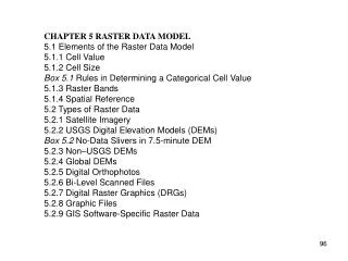
Chapter Outline 7.1 Introduction 7.2 Elements of the Raster Data Model Box 7.1 Rules in Determining a Categorical Cell Value 7.3 Types of Raster Data 7.3.1 Satellite Imagery 7.3.2 Digital Elevation Models 7.3.2.1 The 7.5-minute DEM Box 7.2 No-Data Slivers in 7.5-minute DEM

E N D
Chapter Outline 7.1 Introduction 7.2 Elements of the Raster Data Model Box 7.1 Rules in Determining a Categorical Cell Value 7.3 Types of Raster Data 7.3.1 Satellite Imagery 7.3.2 Digital Elevation Models 7.3.2.1 The 7.5-minute DEM Box 7.2 No-Data Slivers in 7.5-minute DEM 7.3.2.2 The 30-minute DEM 7.3.2.3 The 1-degree DEM 7.3.2.4 Alaska DEMs 7.3.2.5 Non-USGS DEMs 7.3.2.6 Global DEMs 7.3.3 Digital Orthophotos 7.3.4 Binary Scanned Files 7.3.5 Digital Raster Graphics 7.3.6 Graphic Files 7.3.7 GIS Software-Specific Raster Data
7.4 Data Structure, Data Compression, and Header File 7.4.1 Data Structure 7.4.2 Data Compression 7.4.3 Header File Box 7.3 A Header File Example 7.5 Projection and Geometric Transformation of Raster Data 7.6 Data Conversion 7.7 Integration of Raster and Vector Data Box 7.4 Linking Vector Data with Images
Applications: Raster Data Task 1: Import USGS DEM Data Task 2: View a Satellite Image in ArcMap Task 3: Convert Vector Data to Raster Data
Representation of point, line, and area features in raster format (left) and vector format (right).
This illustration shows elevation grids derived from LIDAR data at the canopy level (a) and the ground level (b). The difference between (a) and (b) is the estimated tree height (c). The process of deriving an elevation grid (or DEM) from LIDAR data is as follows: convert LIDAR data to a TIN (triangulated irregular network), and use linear interpolation to convert the TIN to a grid.
Row 1: 0,0,0,0,1,1,0,0 Row 2: 0,0,0,1,1,1,0,0 Row 3: 0,0,1,1,1,1,1,0 Row 4: 0,0,1,1,1,1,1,0 Row 5: 0,0,1,1,1,1,1,0 Row 6: 0,1,1,1,1,1,1,0 Row 7: 0,1,1,1,1,1,1,0 Row 8: 0,0,0,0,0,0,0,0 The cell-by-cell data structure records each cell value by row and column.
Row 1: 5,6 Row 2: 4,6 Row 3: 3,7 Row 4: 3,7 Row 5: 3,7 Row 6: 2,7 Row 7: 2,7 The run length encoding method records the cell values in runs. Row 1, for example, has two adjacent cells in columns 5 and 6 that are gray or have the value of 1. Row 1 is therefore encoded with one run, beginning in column 5 and ending in column 6. The same method is used to record other rows.
N1, E1, N3, E1, N1, E1, N1, E1, S2, E1, S4, W5 Starting at the lower left cell of the region, the chain codes method records the region’s boundary by using the principal direction and the number of cells. In this example, the recording follows a clockwise direction.
The block codes method works with square blocks. The region in the diagram is divided into three unit square blocks, one 4-square block, and one 25-square block. Each block is encoded with the coordinates of its lower left corner.
The regional quad tree method divides a grid into a hierarchy of quadrants. The division stops when a quadrant is made of cells of the same value (gray or white). A quadrant that cannot be subdivided is called a leaf node. In the diagram, the quadrants are indexed spatially: 0 for NW, 1 for SW, 2 for SE, and 3 for NE. Using the spatial indexing method and the hierarchical quad tree structure, the gray cells can be coded as 02, 032, and so on. See text for more explanation.
A The grid in solid line is a new grid created by transforming the grid in dashed lines. Re-sampling is required to fill the value of each cell in the new grid such as cell A.
On the left is an example of conversion from vector to raster data, or rasterization. On the right is an example of conversion from raster to vector data, or vectorization.
Landsat 7 http://landsat7.usgs.gov/ Terra spacecraft http://terra.nasa.gov/About/ U.S. National Oceanic and Atmospheric Administration (NOAA) http://edcdaac.usgs.gov/1KM/1kmhomepage.html/ AmericaView http://americaview.usgs.gov/index.html/ OhioView http://www.ohioview.org/ SPOT satellite http://www.spot.com/
India’s space program http://www.isro.org/ Japan’s space program http://www.nasda.go.jp/ Space Imaging http://www.spaceimaging.com/ DigitalGlobe http://www.digitalglobe.com/ ERDAS http://www.erdas.com/ ER Mapper http://www.ermapper.com/ USGS DEMs http://mcmcweb.er.usgs.gov/status/dem_stat.html/
Intermap Technologies http://www.intermaptechnologies.com/ ETOPO5 (Earth Topography-5 Minute) http://edcwww.cr.usgs.gov/glis/hyper/guide/etopo5 GTOPO30 http://edcdaac.usgs.gov/gtopo30/gtopo30.html/ GLOBE http://www.ngdc.noaa.gov/seg/topo/globe.shtml/ LizardTech, Inc. http://www.lizardtech.com/