Understanding Fourier Transform in Digital Image Processing
270 likes | 939 Views
The Fourier Transform is crucial in decomposing signals into sinusoidal components. For images, it transforms them into frequency space representations. This lecture explains the significance of Fourier Transform in image processing, its efficiency, and applications like filtering. It delves into the intuition behind periodic functions and the differences between 1-D continuous and discrete Fourier transforms. The lecture covers the definition, properties, and applications of 1-D DFT, along with examples using MATLAB functions fft and ifft. It also explores the linearity, shifting, and circular convolution properties of 1-D DFT, emphasizing the importance of convolution in image processing tasks.

Understanding Fourier Transform in Digital Image Processing
E N D
Presentation Transcript
Digital Image ProcessingLecture 8: Fourier Transform Prof. Charlene Tsai
Introduction • The Fourier Transform is generally used to decompose a signal into various sinusoidal components. • For an image, the output of the transformation is the representation of the image in frequency space, while the input image is the real space equivalent. • In the Fourier space image, each point represents a particular frequency contained in the real domain image. Jean Baptiste Joseph Fourier
Significance • The Fourier Transform allows us to perform tasks which would be impossible to perform any other way; its efficiency allows us to perform other tasks more quickly. • The Fourier Transform provides a powerful alternative to linear spatial filtering; it is more efficient to use the Fourier transform than a spatial filter for a large filter. • The Fourier Transform also allows us to isolate and process particular image frequencies, and so perform low-pass and high-pass filtering with a great degree of precision.
Some Intuition • A periodic function may be written as the sum of sines and cosines of varying amplitudes and frequencies. Examples =>
Some Intuition • Some functions will require only a finite number of functions in their decomposition; others will require an infinite number.
1-D Continuous • f(x) is a linear combination of simple periodic patterns. • Where Spatial frequency (measured in whole cycle per unit of x) Simple periodic patterns Inverse Fourier transform Weight function for the given frequency Image co-ordinate Fourier transform
1-D Discrete (con’d) • In image processing, we deal with a discrete function. • Since we only have to obtain a finite number of values, we only need a finite number of functions to do it. • For example:1 1 1 1 -1 -1 -1 -1, which we may take as a discrete approximation to the square wave of figure (a). This can be expressed as the sum of two sine functions, (b) and (c) (a) (b) (c)
Definition of 1-D DFT Suppose is a sequence of length N. Define its discrete Fourier transform where We can express this definition as matrix multiplication Where F is an NxN matrix defined by
Definition of 1-D DFT Given N, we shall define So that Then we can write
Suppose so that N=4. Then Example Then we have
The Inverse DFT Inverse DFT: Difference with forward transform: (1). There is no scaling factor 1/N (2). The sign inside the exponential function has been changed to positive Inverse DFT can also be expressed as matrix product where
Matlab Functions: fft/ifft • Example: » a=[1 2 3 4 5 6 7 8 9] » b=fft(a) 45.0 -4.5 +12.3i -4.5 + 5.3i -4.5 + 2.5i -4.5 + 0.7i -4.5 - 0.7i -4.5 - 2.5i -4.5 - 5.3i -4.5 -12.3i » ifft(b) 1.0 - 0.0i 2.0 - 0.0i 3.0 - 0.0i 4.0 - 0.0i 5.0- 0.0i 6.0 - 0.0i 7.0 + 0.0i 8.0 + 0.0i 9.0 + 0.0i
Properties of 1-D DFT • Linearity:Suppose f and g are two vectors of same length, and p and q are scalars, with h = pf + qg. If F,G and H are the DFT’s of f,g and h, then • Shifting: Suppose we multiply each element xn of a vector x by (-1)n i.e., we change the sign of every second element. Let the resulting vector be denoted x’. Then DFT X’ of x’ is equal to the DFT X of x with the swapping of the left and right halves. H = pF + qG Applications of some of the properties are shown in next lecture
Example » x = [ 2 3 4 5 6 7 8 1] » x1 = (-1).^[0:7].*x x1 = 2 -3 4 -5 6 -7 8 -1 » X=fft(x') X = 36.0000 -9.6569 + 4.0000i -4.0000 - 4.0000i 1.6569 - 4.0000i 4.0000 1.6569 + 4.0000i -4.0000 + 4.0000i -9.6569 - 4.0000i » X1=fft(x1') X1 = 4.0000 1.6569 + 4.0000i -4.0000 + 4.0000i -9.6569 - 4.0000i 36.0000 -9.6569 + 4.0000i -4.0000 - 4.0000i 1.6569 - 4.0000i Then the DFT X1 of x1 is equal to the DFT X of x with the swapping of the left and right halves.
Properties of 1-D DFT (con’d) • Conjugate symmetry:If x is real, and of length N, then its DFT X satisfies the condition ,where is the complex conjugate of for all k=1,2,3,…,N-1. (check out previous slide) • Circular convolution: Suppose x and y are two vectors of the same length N. Then we define their convolution to be the vector, , where
Example Thus
Properties of 1-D DFT (con’d) • Circular convolution: can be defined in terms of polynomial products. • Suppose p(u) the polynomial in u whose coefficients are elements of x. Let q(u) be the polynomial whose coefficients are elements of y. From the product p(u)q(u)(1+uN), and extract the coefficients of uNto u2N-1, these will be the required circular convolution • Example: we have and Then we expand Extracting the coefficients of u4,u5,…., u7 we obtain
Importance of Convolution • Suppose xand yare vectors of equal length. Then the DFT of their circular convolution is equal to the element-by-element product of the DFT's of xand y. • If Z,X,Y are the DFT’s of z=x*y, x and y respectively, then Z=X.Y Example: » fft(cconv(a,b)') ans = 1.0e+002 * 2.6000 -0.0000 - 0.0800i 0.0400 -0.0000 + 0.0800i » fft(a').*fft(b') ans = 1.0e+002 * 2.6000 -0.0000 - 0.0800i 0.0400 -0.0000 + 0.0800i
More on DFT • In general, the transform into the frequency domain will be a complex valued function, that is, with magnitude and phase. • The DC coefficient: The value F(0) average of the input series.
Some Properties of Transform Pair • Scaling relationship: • Time Shift / Frequency Modulation: • The transform of a delta function at the origin is a constant • The transform of a constant function is a DC value only. Unit impulse 1/N f(x) F(u) F(u) f(x)