Stochastic Process - Introduction

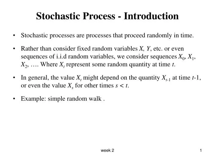
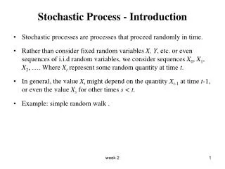
1. Stochastic Process - Introduction • Stochastic processes are processes that proceed randomly in time. • Rather than consider fixed random variables X, Y, etc. or even sequences of i.i.d random variables, we consider sequences X0, X1, X2, …. Where Xt represent some random quantity at time t. • In general, the value Xt might depend on the quantity Xt-1 at time t-1, or even the value Xs for other times s < t. • Example: simple random walk . week 2

2. Stochastic Process - Definition • A stochastic process is a family of time indexed random variables Xt where t belongs to an index set. Formal notation, where I is an index set that is a subset of R. • Examples of index sets: 1) I = (-∞, ∞) or I = [0, ∞]. In this case Xt is a continuous time stochastic process. 2) I = {0, ±1, ±2, ….} or I = {0, 1, 2, …}. In this case Xt is a discrete time stochastic process. • We use uppercase letter {Xt } to describe the process. A time series, {xt } is a realization or sample function from a certain process. • We use information from a time series to estimate parameters and properties of process {Xt }. week 2

3. Probability Distribution of a Process • For any stochastic process with index set I, its probability distribution function is uniquely determined by its finite dimensional distributions. • The k dimensional distribution function of a process is defined by for any and any real numbers x1, …, xk . • The distribution function tells us everything we need to know about the process {Xt }. week 2

4. Moments of Stochastic Process • We can describe a stochastic process via its moments, i.e., We often use the first two moments. • The mean function of the process is • The variance function of the process is • The covariance function between Xt , Xs is • The correlation function between Xt , Xs is • These moments are often function of time. week 2

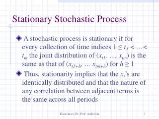
5. Stationary Processes • A process is said to be strictly stationary if has the same joint distribution as . That is, if • If {Xt } is a strictly stationary process and then, the mean function is a constant and the variance function is also a constant. • Moreover, for a strictly stationary process with first two moments finite, the covariance function, and the correlation function depend only on the time difference s. • A trivial example of a strictly stationary process is a sequence of i.i.d random variables. week 2

6. Weak Stationarity • Strict stationarity is too strong of a condition in practice. It is often difficult assumption to assess based on an observed time series x1,…,xk. • In time series analysis we often use a weaker sense of stationarity in terms of the moments of the process. • A process is said to be nth-order weakly stationary if all its joint moments up to order n exists and are time invariant, i.e., independent of time origin. • For example, a second-order weakly stationary process will have constant mean and variance, with the covariance and the correlation being functions of the time difference along. • A strictly stationary process with the first two moments finite is also a second-ordered weakly stationary. But a strictly stationary process may not have finite moments and therefore may not be weakly stationary. week 2

7. The Autocovariance and Autocorrelation Functions • For a stationary process {Xt }, with constant mean μ and constant variance σ2. The covariance between Xt and Xt+s is • The correlation between Xt and Xt+s is Where • As functions of s, γ(s)is called the autocovariance function and ρ(s) is called the autocorrelation function (ATF). They represent the covariance and correlation between Xt and Xt+s from the same process, separated only by s time lags. week 2

8. Properties of γ(s) and ρ(s) • For a stationary process, the autocovariance function γ(s) and the autocorrelation function ρ(s) have the following properties: • . • . • The autocovariance function γ(s) and the autocorrelation function ρ(s) are positive semidefinite in the sense that for any real numbers week 2

9. Correlogram • A correlogram is a plot of the autocorrelation function ρ(s) versus the lag s where s = 0,1, …. • Example… week 2

10. Partial Autocorrelation Function • Often we want to investigate the dependency / association between Xt and Xt+k adjusting for their dependency on Xt+1, Xt+2,…, Xt+k-1. • The conditional correlation Corr(Xt, Xt+k| Xt+1, Xt+2,…, Xt+k-1) is usually referred to as the partial correlation in time series analysis. • Partial autocorrelation is usually useful for identifying autoregressive models. week 2

11. Gaussian process • A stochastic process is said to be a normal or Gaussian process if its joint probability distribution is normal. • A Gaussian process is strictly and weakly stationary because the normal distribution is uniquely characterized by its first two moments. • The processes we will discuss are assumed to be Gaussian unless mentioned otherwise. • Like other areas in statistics, most time series results are established for Gaussian processes. week 2

12. White Noise Processes • A process {Xt} is called white noise process if it is a sequence of uncorrelated random variables from a fixed distribution with constant mean μ (usually assume to be 0) and constant variance σ2. • A white noise process is stationary with autocovariance and autocorrelation functions given by …. • A white noise process is Gaussian if its joint distribution is normal. week 2

13. Estimation of the mean • Given a single realization {xt} of a stationary process {Xt}, a natural estimator of the mean is the sample mean which is the time average of n observations. • It can be shown that the sample mean is unbiased and consistent estimator for μ. week 2

14. Sample Autocovariance Function • Given a single realization {xt} of a stationary process {Xt}, the sample autocovariance function given by is an estimate of the autocivariance function. week 2

15. Sample Autocorrelation Function • For a given time series {xt}, the sample autocorrelation function is given by • The sample autocorrelation function is non-negative definite. • The sample autocovariance and autocorrelation functions have the same properties as the autocovariance and autocorrelation function of the entire process. week 2

16. Example week 2