Building Aware Flow and T&D Modeling Sensor Data Fusion
250 likes | 431 Views
Building Aware Flow and T&D Modeling Sensor Data Fusion. NCAR/RAL March 23 2007. Building Effects. SSW. S. A. SSE. Building Effects. SE. ESE. E. ENE. B. NE. NNE. C. N.

Building Aware Flow and T&D Modeling Sensor Data Fusion
E N D
Presentation Transcript
Building Aware Flow and T&D ModelingSensor Data Fusion NCAR/RAL March 23 2007
Building Effects SSW S A SSE Building Effects SE ESE E ENE B NE NNE C N Arrows indicate flow around typical building structures for an undisturbed wind flowing from left to right. Plume predictions based upon measurements taken at points A, B, or C will indicate transport opposite the mean flow. Example comparing rooftop anemometer to lidar observations.
Building-Aware Model Physical model of Lower Manhattan Laser Doppler velocimeter to measure flows 1:200 scale wind tunnel model EPA Fluid Modeling Facility
QUIC-Urb • Los Alamos developed empirical flow distortion mass consistent model calibrated with wind tunnel experiments • Computes mean, time-averaged, effects of buildings on the wind field • Capable of running at a resolution of a few meters
QUIC-Urb • Buildings are composed of rectilinear blocks that are an integer number of grid cells • Buildings superimposed within the unmodified wind field • Empirical algorithms are used to estimate the velocities in various zones around the buildings - the zones are a function of the size of the building and wind speed and direction
QUIC-Urb • A diagnostic wind scheme, continuity, is used to adjust the winds to account for mass conservation and obstacle blocking effects • Allows for realistic rotational flow • Frozen hydrodynamics - change of flow with time is obtained through successive application of the whole process
QUIC-Urb • Building elements should maximize horizontal area. Unrealistic flows can arise from improper building construction. • Complicated building shapes can be built from simple rectilinear elements
Lagrangian Particle Modeling • Stochastic model of Lagrangian velocities (Monte-Carlo, Markov-chain) Particles move with the mean wind plus perturbation Perturbation is part memory part turbulence Memory coefficient • Eulerian mean and turbulent fields - From a mesoscale, LES, or CFD model • t generally given by x, y, or z - From model or parameterized • t is a dimensionless random variable with mean of 0 and variance of 1 • TL is the integrated Lagrangian time scale
Lagrangian Particle Modeling Building reflection Concentration computation • Each particle represents a finite amount of material • Concentration based on sum of particles within a grid cell • Account for buildings by reflection of particles off building surfaces • How many particles to use? • Statistical significance • Size of grid cells • Distance from source • Strength of turbulence • Available run time
Lagrangian Particle Modeling • Advantages • Modifications for inhomogeneous turbulence • Complicated sources/releases • Treatment of buildings reasonably simple • Disadvantages • Number of particles (runtime, concentration) • Complications dealing with chemical reactions • Hybrids • Langrangian Puff • Langrangian/Eulerian
QUIC-Plume • Building aware Lagrangian particle dispersion model developed by Los Alamos National Lab • Building aware wind field input from QUIC-Urb Example of QUIC-Plume running over a multi building urban area.
Lagrangian-Puff Modeling (SCIPUFF/HPAC) Puff concentration • Concentration field represented by collection of 3-D puffs • Puffs characterized by 3-moments of the puff concentration • 0th Mass • 1st Centroid • 2nd Spread Q + • Lagrangian transport of Gaussian puffs
Lagrangian-Puff Modeling SPLIT Boundary MERGE • Develop prognostic equations for each of the moments based upon environmental conditions • Assume that environmental conditions at puff centroid are representative for whole puff • Splitting and merging of puffs • Instantaneous or continuous releases, sources from 3rd party models • Reflection of puffs at boundaries - difficulties for treatment of buildings • Buildings treated as additional surface roughness (Urban Wind Model - UWM) • Urban Dispersion Model - UDM
SCIPUFF Typical HPAC plume using VLAS wind field. Example of building effects in HPAC. This simulation did not execute in an emergency response time frame.
Sensor Data Fusion • Scenario • A sensor or sensor network detects CBR materials CBR Sensor Location
Sensor Data Fusion • Scenario • A sensor or sensor network detects CBR materials • Detection is currently used as the source to forecast the downwind impact CBR Sensor Location Sensor Detection Based Plume
Sensor Data Fusion Actual Release Location CBR Sensor Location Sensor Detection Based Plume • Scenario • A sensor or sensor network detects CBR materials • Detection is currently used as the source to forecast the downwind impact • This forecast may not accurately reflect the actual threat
Sensor Data Fusion • Scenario • A sensor or sensor network detects CBR materials • Detection is currently used as the source to forecast the downwind impact • This forecast may not accurately reflect the actual threat Actual Release Location Actual CBR Plume CBR Sensor Location Sensor Detection Based Plume
CBR SDF Objective • Given disparate CBR sensor readings and meteorological measurements, determine: • CBR Source Characteristics (Location, Mass, Time) • CBR Refined Downwind Hazard (Surface Dosage) Source Characterization CB/Met Sensors SDF Refined Downwind Hazard • Essentially this is done by using sensor readings at sources and running the T&D model in reverse (adjoint) • Then determine PDF of reverse concentration peaks (most likely location of source) • Complications - Continuous sources, multiple sources, moving sources
Demonstration Control Experiment: Single Source, Perfect Sensors, Known Release Time
Demonstration Control Experiment: Single Source, Perfect Sensors, Known Release Time
Demonstration Control Experiment: Single Source, Perfect Sensors, Known Release Time
Demonstration Control Experiment: Single Source, Perfect Sensors, Known Release Time
Demonstration Control Experiment: Single Source, Perfect Sensors, Known Release Time
Demonstration Control Experiment: Single Source, Perfect Sensors, Known Release Time

![Data Modeling [Comparison of data modeling techniques ]](https://cdn0.slideserve.com/205866/data-modeling-comparison-of-data-modeling-techniques-dt.jpg)