Download
1 / 57
610 likes | 828 Views
Biostatistics I PubH 6450. Fall 2005. PubH 6450 – Biostatistics I. Instructor: Susan Telke email: susant@biostat.umn.edu (office hours: 3:20pm – 4:20pm (T and TH), location – lecture hall or by appointment, location -A349 Mayo building) Teaching Assistants:

E N D
Biostatistics IPubH 6450 Fall 2005
PubH 6450 – Biostatistics I Instructor: Susan Telke email: susant@biostat.umn.edu (office hours: 3:20pm – 4:20pm (T and TH), location – lecture hall or by appointment, location -A349 Mayo building) Teaching Assistants: Pei Li – email: peili@biostat.umn.edu Xiaoxiao Kong – email: xiaoxiak@biostat.umn.edu Jianmin Liu – email: jianminl@biostat.umn.edu Xiaobo Liu – email: xiaobol@biostat.umn.edu Ran Li – email: ranli@biostat.umn.edu Jia Xu – email: jiaxu@biostat.umn.edu Jay Pottala – email: jamesp@biostat.umn.edu
Book for 6450 Introduction to the Practice of Statistics -(Moore and McCabe)
Web Page http://www.biostat.umn.edu/~susant/PH6450DESC.html Information on the web: • General class information • Syllabus • Course notes (updated weekly) • Homework • Computer Help
Computer Labs • Mayo C381 (Biostatistics Lab) Teaching Assistants will have computer sessions located in the mayo lab to help you with your homework assignments. • Deihl Hall (Medical Library)
PC SAS Primary computing environment will be PC SAS • PC SAS is available in computing lab MAYO C381 • PC SAS can be purchased at the bookstore (one year agreement is about $50). • SAS (not PC SAS) is available using the UNIX version of SAS by telnet to the biostat workstation saturn.
Exams and Homework • There will be weekly homework assignments • There will be two midterms and one final exam. • Students who get an “A” on all exams get an “A” in the course. • For all other students the midterms account for 25% each and the final accounts for 30% of the course grade. The remaining 20% is based on homework (best 9)
Introduction to PubH 6450 • The study of statistics explores the collection, organization, analysis and interpretation of numerical data. • When the focus of the analysis is on the biological and health sciences it is called Biostatistics.
Trial by Jury:A Familiar Scenario • You have a crime. • You have a suspect. • A police investigation collects evidence against the suspect. • A prosecutor presents summarized evidence to a jury.
Trial by Jury:The Process • The Jury reaches a verdict based on their judgment of the evidence presented. • Rules for determining a verdict: • The accused is innocent until proven guilty • The evidence must be sufficient to convict beyond all reasonable doubt • Decision must be unanimous
Trial by Jury:The Need Why is the Trial by Jury process needed? The truth is unknown or uncertain because of : • Variability: Every case is different. • Incomplete information: Some evidence may be missing.
Trial by Jury:Rationale • Trial by Jury is the way our society deals with uncertainties related to criminal justice. • Its goal is to minimize errors/mistakes within the limits of human understanding. • It is impossible to eliminate all mistakes in verdicts made based on uncertain, incomplete evidence.
Trial by Jury:Dealing with Uncertainty • A hypothesis (assumption) is stated: “Every person is innocent until proven guilty” • Data is collected: Evidence against the hypothesis – not against the suspect. • A verdict is reached based on the evidence about whether the hypothesis should be rejected. (If hypothesis rejected – verdict is guilty)
Trial by Jury:Elements of a Successful Trial • A probable cause (a crime and a suspect). • A thorough investigation (by police). • An efficient presentation (by D.A.’s office attorneys – organization and summarization of evidence). • A fair & impartial assessment by the jury.
Trial by Jury:How does this relate to Biostatistics? • A probable cause: The crime is lung cancer & the suspect is cigarette smoking. • A thorough investigation: A clinic trial or case control study to gather information. • An efficient presentation: Using biostatistics tools to organize and summarize data. • A fair & impartial assessment by the jury: Making proper statistical inference based on data collected.
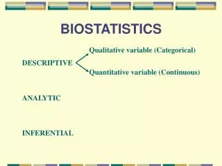
Areas of Biostatistics Experimental Designs: How will the data be collected? Descriptive Statistics: Organization of data Summary statistics of data Effective graphical representation of data Statistical Inference The science of drawing statistical conclusions from specific data using a knowledge of probability.
Goals … By the end of the course you should be able to use the following aspects of statistical thinking: • Critically read the literature in your field that makes use of statistical analysis. • Read about new statistical techniques and understand how they may apply to your field. • Create and analyze descriptive statistics based on data. • Develop hypotheses and use appropriate statistics to evaluate these hypotheses.
The Language of Statistics:Definitions • Population: The entire group of people, animals or things about which we want information. (e.g. population of the U.S.) • Individuals(units): The objects described by a set of data. (e.g. People) • Sample: A part of the population from which we actually collect information, used to draw conclusions about the whole population. (e.g. sample=1000 people)
The Language of Statistics:Definitions • Variable: Any characteristic of an individual. A variable can take different values for different individuals. Also, a variable can take different values for the same individual at different times. (e.g. Height, age, gender)
Two “Types” of Variables • Quantitative Variable: measures that are recorded on a naturally occurring numerical scale. Operations such as adding and “averaging” make sense. (e.g. Height, time, test scores) • Qualitative Variable (Categorical): Variables that are classified into one of a group of categories. Arithmetic operations do NOT make sense with this type of variable. (e.g. Geographical location, gender)
Examples: • Age in years • ID # • Temperature in degrees • Political party • Smoking status • Length in cm • Gender • Blood pressure
Two Methods for Describing Sets of Data Exploratory Data analysis: examining data in order to describe their main features. Graphical Numerical
Displaying Distributions with Graphs • Distribution: The distribution of a variable tells us what values it takes on and how often it takes on these values.
Describing Categorical Variables with Graphs Bar Graphs NOTE: 668 children living in crack/cocaine households were categorized based on race
Describing Categorical Variables with Graphs Pie Chart NOTE: 668 children living in crack/cocaine households were categorized based on race
Describing Quantitative Data • Stemplots • Histograms • Time Plots • Box Plots (section 1.2)
Stemplots Quick easy way to see distribution of 40 or less data points • How to make a stemplot • Create Leaf • Order Data • Arrange Stems • Place Leaves
Stemplots:An Example Average Monthly Temperature. Source: World Almanac 1996 p.180
Histograms • Histograms are useful to display the distribution of large amounts of data. • Steps for creating a histogram • Divide range into classes of equal width • Count number of observations in each class • Draw histogram
Histogram:An Example • Weights of 92 Penn State Students: • Females 140 120 130 138 121 125 116 145 150 112 125 130 120 130 131 120 118 125 135 125 118 122 115 102 115 150 110 116 108 95 125 133 110 150 108 • Males 140 145 160 190 155 165 150 190 195 138 160 155 153 145 170 175 175 170 180 135 170 157 130 185 190 155 170 155 215 150 145 155 155 150 155 150 180 160 135 160 130 155 150 148 155 150 140 180 190 145 150 164 140 142 136 123 155
Number of Intervals • There is no clear-cut rule on the number of intervals or classes that should be used. • Too many intervals – the data may not be summarized enough for a clear visualization of how they are distributed. • Too few intervals – the data may be over-summarized and some of the details of the distribution may be lost.
Pictures of Data: Histograms • Blood pressure data on a sample of 113 men Histogram of the Systolic Blood Pressure for 113 men. Each bar spans a width of 5 mmHg on the horizontal axis. The height of each bar represents the number of individuals with SBP in that range.
Pictures of Data: Histograms Another histogram of the blood pressure of 113 men. In this graph, each bar has a width of 20 mmHg, and there are a total of only 4 bars making it hard to characterize the distribution of blood pressures in the sample.
Pictures of Data: Histograms Yet another histogram of the same BP information on 113 men. Here, the bin width is 1 mmHg, perhaps giving more detail than is necessary.
Width of Intervals • Without some specific reason (i.e. showing infant death) the intervals should all be the same width. • Common width =W= • R = range of the data • k = the number of intervals
Consideration when Determining Width • Width should be chosen so that it is convenient to use or easy to recognize (multiples of 5 or 1). • The beginning of the first interval must be low enough so that the first interval includes the smallest observation. • If the data has x decimal places, the interval limits should also have x decimal places.
Data Example • Weight in pounds of 57 school children at a day-care center: 68 63 42 27 30 36 28 32 79 27 22 23 24 25 44 65 43 23 74 51 36 42 28 31 28 25 45 12 57 51 12 32 49 38 42 27 31 50 38 21 16 24 69 47 23 22 43 27 49 28 23 19 46 30 43 49 12
Data Example – Step 1 • From the data we have: • Minimum = 12 • Maximum = 79 • R = 79-12 = 67 • If we use k=5 and 15 we get: • W= 69/5 = 13.4 • W= 69/15 = 4.5 • Since the dataset is not large, we will choose w=10 to have fewer intervals.
Data Example – Step 2 • Next we have to construct the intervals. • With w = 10 and minimum=12 choose the first interval to start at 10. INTERVALS (in lbs): 10-19 20-29 30-39 40-49 50-59 60-69 70-79
Data Example – Step 3 Examine the values one at a time and tally the number in each interval.
Data Example – Step 4 Calculate Relative Frequencies: Relative freq. = frequency in interval # obs in dataset
Histogram • Horizontal scale represents the value of the variable • The vertical scale represents the frequency or relative frequency in each interval • Rectangular bars are joined together
Consider Distibutions • If the data are homogeneous, the graphs usually show a unimodal pattern with one peak in the middle. • The plots can be used to determine if the data is symmetric. A symmetric distribution is one in which the distribution has the same shape on both sides of the peak.
Shapes of the Distribution • Three common shapes of frequency distributions: A B C Symmetrical and bell shaped Positively skewed or skewed to the right Negatively skewed or skewed to the left