Download
1 / 46
470 likes | 1.26k Views
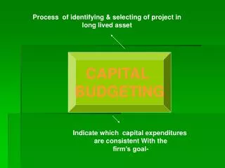
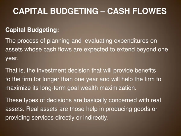
Capital budgeting involves making long-term investment decisions to determine if the benefits of a project justify the initial outlay. The process requires careful planning and evaluation due to factors such as irreversibility and uncertainty in the business landscape.

E N D
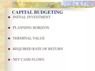
Capital budgeting • It is a decision involving selection of capital expenditure proposals. • The life of the project is atleast one year and usually much longer. • Examples include decision to purchase new plant and equipment • Introduce new product in the market • Essentially it must be determined whether the future benefits are sufficiently large enough to justify the current outlays.
Capital budgeting • A capital budgeting decision is one that involves the allocation of funds to projects that will have a life of atleast one year and usually much longer. • Examples would include the development of a major new product, a plant site location, or an equipment replacement decision. • Capital budgeting decision must be approached with great care because of the following reasons: • Long time period: consequences of capital expenditure extends into the future and will have to be endured for a longer period whether the decision is good or bad.
Substantial expenditure: it involves large sums of money and necessitates a careful planning and evaluation. • Irreversibility: the decisions are quite often irreversible, because there is little or no second hand market for may types of capital goods. • Over and under capacity: an erroneous forecast of asset requirements can result in serious consequences. First the equipment must be modern and secondly it has to be of adequate capacity.
Difficulties • There are three basic reasons why capital expenditure decisions pose difficulties for the decision maker. These are: • Uncertainty: the future business success is today’s investment decision. The future in the real world is never known with certainty. • Difficult to measure in quantitative terms: Even if benefits are certain, some might be difficult to measure in quantitative terms. • Time Element: the problem of phasing properly the availability of capital assets in order to have them come “on stream” at the correct time.
Decision process INVESTMENT OPPORTUNITIES PROPOSALS PLANNING PHASE REJECTED OPPORTUNITIES Improvement in planning & Evaluation procedure Improvement in planning & Evaluation procedure PROPOSALS NEW INVESTMENT OPPORTUNITIES EVALUATION PHASE Rejected Proposals PROJECTS SELECTION PHASE Rejected projects ACCEPTED PROJECTS IMPLEMENTATION PHASE ONLINE PROJECTS CONTROL PHASE PROJECT TERMINATION AUDITING PHASE
Methods of classifying investments • Independent • Dependent • Mutually exclusive • Economically independent and statistically dependent independent Mutual Exclusive Prerequisite Weak complement Strong substitute Weak substitute Strong complement
Profit (Service) Maintaining and profit (service) adding investment • Investment may fall into two basic categories, profit-maintaining and profit-adding when viewed from the perspective of a business, or service maintaining and service-adding when viewed from the perspective of a government or agency.
Option for replacement decision How long? What problems? Can we go on? Are there better opportunities? Is the product life coming to an end? Go out of business Do nothing Replace with same What if volume increases? How secure are the markets? Replace larger or smaller Replace different process Should a margin of capacity Be provided? Present point Of decision Can we profit from new technology? What risks are there? Etc. Etc.
Expansion and new product investment • Expansion of current production to meet increased demand • Expansion of production into fields closely related to current operation – horizontal integration and vertical integration. • Expansion of production into new fields not associated with the current operations. • Research and development of new products.
Reasons for using cash flows • Economic value of a proposed investment can be ascertained by use of cash flows. • Use of cash flows avoids accounting ambiguities • Cash flows approach takes into account the time value of money
Incremental cash flows • For any investment project generating either expanded revenues or cost savings for the firm, the appropriate cash flows used in evaluating the project must be incremental cash flow. • The computation of incremental cash flow should follow the “with and without” principle rather than the “before and after” principle
Investment decision Cash Investment Opportunity (real asset) Investment Opportunities (financial assets) shareholder Firm Alternative: Pay dividend To shareholders Shareholders Invest for themselves invest
Different methods of measurement • Payback • Average return on book value • Net present value • Internal rate of return • Profitability index
NPV • NPV rule recognizes that a dollar today is worth more than a dollar tomorrow, because the dollar today can be invested to start earning interest immediately. • Any investment rule which does not recognize the time value of money cannot be sensible • NPV depends solely on the forecasted cash flows from the project and the opportunity cost of capital • Because the present values are all measured in today’s dollars, you can add them up.
If you have two projects A and B, the net present value of the combined investment is : • NPV(A+B) = NPV(A) + NPV(B) • This additive property has important implications. Suppose project B has a negative NPV. If you tack it onto project A, the joint project (A+B) will have a lower NPV than A on its own. Therefore, you are unlikely to be misled into accepting a poor project (B) just because it is packaged with a good one (A).
Payback • Companies frequently require that the initial outlay on any project should be recoverable within some specified cutoff period. • The payback period of a project is found by counting the number of years it takes before cumulative forecasted cash flows equal the initial investment.
Cash flows, dollars Consider project A and B :
-$182 2,000 1.10 = NPV(A) = -2,000 + 1,000 (1.10)3 1,000 1.10 1,000 (1.10)2 +$3492 + + NPV(B) = -2,000 + = Thus the net present value rule tells us to reject project A and accept project B.
The payback rule says that these projects are all equally attractive. But project B has a higher NPV than project C for any positive interest rate ($1,000 in each of years 1 and 2 is more valuable than $2,000 in year 2). And project D has a higher NPV than either B or C. • In order to use the payback rule a firm has to decide on an appropriate cutoff date. If it uses the same cutoff regardless of project life, it will tend to accept too many short-lived projects and too few long-lived ones. If, on average, the cutoff periods are too long, it will accept some projects with negative NPVs; if, on average, they are too short, it will reject some projects that have positive NPVs.
Discounted Payback • Some companies discount the cash flows before they compute the payback period. The discounted payback rule asks, “How many periods does the project have to last in order to make sense in terms of net present value? • The discounted cash flow surmounts the objection that equal weight is given to all flows starting in year1. The cash flow for investment before the cut off date. • The discounted payback rule still takes no account of any cash flows after the cutoff date.
Example of Discounted payback method • Suppose there are two mutually exclusive investments, A and B. Each requires a $20,000 investment and is expected to generate a level stream of cash flows starting in year 1. The cash flow for investment A is $6,500 and lasts for 6 years. The cash flow for B is $6,000 but lasts for 10 years. The appropriate discount rate for each project is 10 percent. Investment B is clearly a better investment on the basis of net present value:
NPV(A) = -20,000 + ∑6t=1 6,500 = + $8,309 (1.10) t NPV(B) = -20,000 + ∑10t=16,000 = + $16,867 (1.10) t Yet A has higher cash receipts than B in each year of its life, and so obviously A has the shorter discounted payback. The discounted Payback of B is a bit more than 4 years, since the present value of $6,000 for 4 years is $19,019. Discounted payback is a whisker better than undiscounted payback.
Average return on book value • Some companies judge an investment project by looking at its book rate of return. • To calculate book rate of return it is necessary to divide the average forecasted profits of a project after depreciation and taxes by the average book value of the investment. • This ratio is then measured against the book rate of return for the firm as a whole or against some external yardstick, such as the average book rate of return for the industry.
Computing the average book rate of return on an investment of $9,000 in project A Avg. book rate of return • avg. annual • income • avg.annual investment = = 2,000 = .44 4,500
Internal rate of return Alternatively, we could write down the NPV of the investment and find that discount rate which makes NPV = 0 Implies Discount rate = payoff _______________ - 1 Investment Rate of return = C1 _______________ = 0 1 + discount rate NPV = Co + C1 - 1 - C0
C1 is the payoff and –C0 the required investment, and so our two equations say exactly the same thing. The discount rate that makes NPV= 0 is also the rate of return. Unfortunately there is no wholly satisfactory way of defining the true rate of return of a long-lived asset. The best available concept is the so-called discounted cash-flow (DCF) rate of return or internal rate of return (IRR). The internal rate of return is frequently used in finance. The internal rate of return is defined as the rate of discount which makes NPV=0. This means that to find the IRR for an investment project lasting T years, we must solve for IRR in the following expression: NPV = C0 + C1 + C1 + C1 + ….. + CT= 0 1 + IRR(1 + IRR)2(1 + IRR)3 (1 + IRR)T Actual calculation of IRR usually involves trial and error. For example, consider a project which produces the following flows:
The internal rate of return is IRR in the equation NPV = - 4,000 + 2,000 + 4,000 = 0 1+ IRR (1 + IRR)2 Let us arbitrarily try a discount rate of 25 percent. In this case NPV = - 4,000 + 2,000 + 4,000 = + $160 1.25 (1. 25)2
The NPV is positive; therefore, the IRR must be greater than zero. The next step might be to try a discount rate of 30 percent. In this case net present value is : • NPV = - 4,000 + 2,000 + 4,000 = - 94 1.30 (1.30)2 In this case net present value is – 94: Therefore the IRR must lie between the rate of 25 and 30. we can find the rate by interpolation. 25 + 5 X 160 = 25 +5 X 160 160 – (-94) 254 = 28.15 percent is the IRR
Profitability index • The profitability index ( or the benefit cost ratio) is the present value of forecasted future cash flows divided by the initial investment: • Profitability index = PVCi PVC0 The profitability index rule tells us to accept all projects with an index greater than 1. If the profitability index is greater than 1, the present value PV of Ci is greater than the initial investment - C0 and so the project must have a positive net present value.
Profitability index • The benefit cost ratio in the case of previous example at the discount rate of 25 percent would be 4160 4000 1.04 =
Time value of money • In 1624, the Indians sold Manhattan Island at the ridiculously low figure of $24. • Was the amount really ridiculous? • If the Indians had merely taken the $24 and reinvested it at 6 percent annual interest upto 1992, they would have had $50 billion, an amount sufficient to repurchase most of New York City. • If the Indians had been slightly more astutute and had invested the $24 at 7.5% compound annually, they would now have over $8 trillion and the tribal chiefs would now rival oil sheikhs and Japanese tycoons as the richest people in the world.
Another popular example is that $1 received 1,992 years ago, invested at 6 % could now be used to purchase all the wealth in the world. • Time value of money applies to day to day decisions. • Understanding the effective rate on a business loan • The mortgage payment in a real estate loan • Distinction must be made on money received today and money received in the future.
Future value • Assume that an investor has $1000 and wishes to know its worth after four years if it grows at 10 percent per year. At the end of the first year, he will have $1000 X 1.10 or 1,100. By the end of the year two, the $1,100 will have grown to $1,210 ($1,100 X 1.10). The four-year pattern is indicated below.
1st year $1,000 X 1.10 = $1,100 • 2nd year $1,100 X1.10 = $1,210 • 3rd year $1,210 X1.10 = $1,331 • 4th year $1,331 X 1.10 = $1,464 If: • FV = Future value • PV = Present value • i = Interest rate • n = Number of periods • The formula for calculation of FV = PV(1+i)n • In this case PV = $1,000, I = 10%, n=4, so we have • FV = $1,000(1.10)4 or $1,000 X 1.464 = $1,464
Relationship of present value and future value 2 $1,464future value $ 10 % interest $1000 Present value 0 1 3 4 Number of periods
Present value • The formula for the present value is derived from the original formula for future value • FV = PV(1+i)n -------Future Value • PV = FV[1/(1+i)n] -----Present Value • The present value of $1,464 in the previous example is $1,000 today that is it is calculated as follows: • PV= FV X PVif (n =4, I= 10%) if = interest factor as given in the chart • PV = $1,464 X 0.683 = $1,000
Compounding process of annuity Period 4 Period 1 Period 2 Period 3 Period 0 $1,000 X 1.000 = $1,000 $1,000 for one period – 10% $1,000 X 1.100 = $1,100 $1,000 for two periods – 10% $1,000 X 1.210 = $1.210 $1,000 for three periods – 10% $1,000 X 1.331 = $1.331 $4,641 To find the present value of annuity the process is reversed.In theory, each individual paymentis discounted back to the present and then all of the discounted payments are added up, yielding the present value of annuity.
The relationship between the present value and future value • It would be noticed that the future value and the present value are the flip side of each other. • Because you can earn a return on your money, $1.00 received in the future is less than $1.00 today, and the longer you have to wait to receive the dollar, the less it is worth. • Because we want to avoid large mathematical rounding errors, we actually carry the decimal points 3 places. For example $.683
Future value for say $.68 at 10 – Graphical presentation 1.00 Value at the end of each period 1.00 .909 0.90 .826 0.80 .751 0.70 .683 0.60 0.00 Period 0 Period 1 Period 2 Period 3 Period 4
Present value of $1.00 at 10% • Value at the beginning of each period 1.00 1.00 0.90 .909 0..80 .826 0.70 .751 .683 0.60 1.00 Period 0 Period 1 Period 2 Period 3 Period 4
The PV of a 2 year annuity is simply the present value of one payment at the end of period 1 and one payment at the end of Period 2 PV of a 4 year annuity 3.17 3.00 PV of $1.00 to be received In 1 year $3.50 .909 2.50 2.49 PV of $1.00 to be received In 2 years .826 2.00 .909 1.74 1.50 .909 .826 .751 PV of $1.00 to be received In 3 years 1.00 .909 .909 0.50 .826 .751 .683 PV of $1.00 to be received In 4 years 0.00 Period 1 Period 2 Period 3 Period 4
Relationship between the PV of a single amount and the present value of an annuity • The relationship between the present value of $1.00 and the present value of a $1.00 annuity. The assumption is that you will receive $1.00 at the end of each period. This is the same concept as a lottery, where you win $2 million over 20 years and receive $100,000 per year for twenty years.
PV of a 4 year annuity $5.00 The PV of a 2 year annuity is simply the future value of one payment at the end of period 1 and one payment at the end of Period 2 4.641 $4.50 PV of $1.00 invested at the end of Period 4 $3.50 1.00 3.00 Future value of an annuity of $1.00 at 10% 2.50 3.31 PV of $1.00 invested for 1 year 1.10 1.00 2.10 2.00 1.50 1.00 .1.10 1.21 PV of $1.00 invested for 2 years 1.00 1.00 1.00 1.10 .1.21 0.50 .1.33 PV of $1.00 invested For 3 years 0.00 Period 1 Period 2 Period 3 Period 4