Download
1 / 44
440 likes | 472 Views
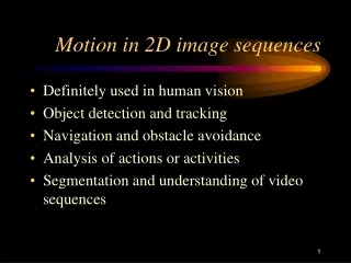
Motion in 2D image sequences. Definitely used in human vision Object detection and tracking Navigation and obstacle avoidance Analysis of actions or activities Segmentation and understanding of video sequences. Frame from an ARDA Sample Video. Change detection for surveillance.

E N D
Motion in 2D image sequences • Definitely used in human vision • Object detection and tracking • Navigation and obstacle avoidance • Analysis of actions or activities • Segmentation and understanding of video sequences
Change detection for surveillance • Video frames: F1, F2, F3, … • Objects appear, move, disappear • Background pixels remain the same • Subtracting image Fm from Fn should show change in the difference • Change in background is only noise • Significant change at object boundaries
Person detected entering room Pixel changes detected as difference regions (components). Regions are (1) person, (2) opened door, and (3) computer monitor. System can know about the door and monitor. Only the person region is “unexpected”.
Change detection via image subtraction for each pixel [r,c] if (|I1[r,c] - I2[r,c]| > threshold) then Iout[r,c] = 1 else Iout[r,c] = 0 Perform connected components on Iout. Remove small regions. Perform a closing with a small disk for merging close neighbors. Compute and return the bounding boxes B of each remaining region.
Change analysis Known regions are ignored and system attends to the unexpected region of change. Region has bounding box similar to that of a person. System might then zoom in on “head” area and attempt face recognition.
Some cases of motion sensing • Still camera, single moving object, constant background • Still camera, several moving objects, constant background • Moving camera, relatively constant scene • Moving camera, several moving objects
Approach to motion analysis • Detect regions of change across video frames Ft and F(t+1) • Correlate region featuresto define motion vectors • Analyze motion trajectoryto determine kind of motion and possibly identify the moving object
Flow vectors resulting from camera motion Zooming a camera gives results similar to those we see when we move forward or backward in a scene. Panning effects are similar to what we see when we turn.
Image flow field • The image flow field (or motion field) is a 2D array of 2D vectors • representing the motion of 3D scene points in 2D space. image at time t image at time t + (sparse) flow field What kind of points are easily tracked?
The Decathlete Game (Left) Man makes running movements with arms. (Right) Display shows his avatar running. Camera controls speed and jumping according to his movements.
Program interprets motion • Opposite flow vectors means RUN; speed determined by vector magnitude. • Upward flow means JUMP. • (c) Downward flow means COME DOWN.
Flow vectors from point matches Significant neighborhoods are matched from frame k to frame k+1. Three similar sets of such vectors correspond to three moving objects.
Examples: First Image Interesting Points Motion Vectors Second Image Interesting Points Clusters
Two aerial phots of a city: MotionVectors First Image Interesting Points Clusters Second Image Interesting Points
Requirements for interest points • Have unique multidirectional energy • Detected and located with confidence • Edge detector not good (1D energy only) • Corner detector is better (2D constraint) • Autocorrelation can be used for matching neighborhood from frame k to one from frame k+1
Interest point detection method • Examine every K x K image neighborhd. • Find intensity variance in all 4 directions. • Interest value is MINIMUM of variances. Consider 4 “1D signals” – horizontal, vertical, diagonal 1, and diagonal 2. Interest value is the minimum variance of these.
Interest point detection algorithmfor window of size w x w for each pixel [r,c] in image I if I[r,c] is not a border pixel and interest_operator(I,r,c,w) threshold then add [(r,c),(r,c)] to set of interest points The second (r,c) is a placeholder for the end point of a vector. procedure interest_operator(I, r, c, w) { v1 = intensity variance of horizontal pixels I[r,c-w]…I[r,c+w] v2 = intensity variance of vertical pixels I[r-w,c]…I[r+w,c] v3 = intensity variance of diagonal pixels I[r-w,c-w]…I[r+w,c+w] v4 = intensity variance of diagonal pixels I[r-w,c+w]…I[r+w,c-w] return minimum(v1, v2, v3, v4) }
Matching interest points P 169 Cross Correlation Can use normalized cross correlation or image difference.
Moving robot sensor 2 views and edges. Bottom right shows overlaid edge images.
MPEG Motion Compression • Some frames are encoded in terms of others. • Independent frame encoded as a still image using JPEG • Predicted frame encoded via flow vectors relative to the independent frame and difference image. • Between frame encoded using flow vectors and independent and predicted frame.
MPEG compression method F1 is independent. F4 is predicted. F2 and F3 are between. Each block of I is matched to its closest match in P and represented by a motion vector and a block difference image. Frames B1 and B2 between I and P are represented by twomotion vectors per block referring to blocks in F1 and F4.
Example of compression • Assume frames are 512 x 512 bytes, or 32 x 32 blocks of size 16 x 16 pixels. • Frame A is ¼ megabytes before JPEG • Frame B uses 32 x 32 =1024 motion vectors, or 2048 bytes only if delX and delY are represented as 1 byte integers.
Computing image flow • Goal is to compute a dense flow field with a vector for every pixel. • We have already discussed how to do it for interest points with unique neighborhoods. • Can we do it for all image points?
Computing image flow Example of image flow: a brighter triangle moves 1 pixel upward from time t1 to time t2. Background intensity is 3 while object intensity is 9.
Optical flow • Optical flow is the apparent flow of intensities across the retina due to motion of objects in the scene or motion of the observer. • We can use a continuous mathematical model and attempt to compute a spatio-temporal gradient at each image point I [x, y, t], which represents the optical flow.
Assumptions for the analysis • Object reflectivity does not change t1 to t2 • Illumination does not change t1 to t2 • Distances between object and light and camera do not change significantly t1 to t2 • Assume continuous intensity function of continuous spatial parameters x,y • Assume each intensity neighborhood at time t1 is observed in a shifted position at time t2.
Image Flow Equation Using the continuity of the intensity function and Taylor series we get: The image flow vector V=[x, y] maps intensity neighborhood N1 of (x,y) at t1 to an identical neighborhood N2 of (x+ x,y+ y) at t2, which yields: Combining we get the image flow equation which gives not a solution but a linear constraint on the flow.
Meaning of image flow equation f - ------ t = f [ δx, δy] t the dot product of the spatial gradient f and the flow vector V = [ δx, δy] the change in the image function f over time =
Computing Image Flow • Colin’s lecture on Wednesday will cover the basics. • I will talk about Ming Ye’s work (see paper)
Segmenting videos • Build video segment database • Scene change is a change of environment: newsroom to street • Shot change is a change of camera view of same scene • Camera pan and zoom, as before • Fade, dissolve, wipe are used for transitions
Detect via histogram change (Top) gray level histogram of intensities from frame 1 in newsroom. (Middle) histogram of intensities from frame 2 in newsroom. (Bottom) histogram of intensities from street scene. Histograms change less with pan and zoom of same scene.
Hierarchical Description of Video Content: MPEG-7 • Definitions of DESCRIPTIONS for indexing, retrieval, and filtering of visual content. • Syntax and semantics of elementary features, and their relations and structure .
Our problem (II): Finding Video Structure • Video Structure: hierarchical description of visual content Table of Contents • From thousands of raw frames to video events
Video Sequence Scenes: Semantic Concept. Fair to use? Clusters: Collection of temporally adjacent/visually similar shots Shots: Consecutive frames recorded from a single camera Sequence Scene Cluster Shot Frame Hierarchical Structure in Video: Extensive Operators
One scenario: home video analysis • Accessing consumer video • Organizing and editing personal memories • The problems: • Lack of Storyline • Unrestricted Content • Random Quality • Non-edited • Changes of Appearance • With/without time-stamps • Non-continuous audio
Our approach • Investigate statistical models for consumer video • Bayesian formulation for video structuting • Encode prior knowledge • Learning models from data • Hierarchical representation of video segments: extensive partition operators. • User interface visualization, correction, reorganization of Table Of Contents
Our Approach VIDEO SEQUENCE TEMPORAL PARTITION GENERATION VIDEO SHOT FEATURE EXTRACTION PROBABILISTIC HIERARCHICAL CLUSTERING CONSTRUCTION OF VIDEO SEGMENT TREE
Video Structuring Results (I) • 35 shots • 9 clusters detected
Video Structuring Results (II) • 12 shots • 4 clusters
Motion analysis on current frontier of computer vision • Surveillance and security • Video segmentation and indexing • Robotics and autonomous navigation • Biometric diagnostics • Human/computer interfaces