Download
1 / 21
210 likes | 340 Views
Ray-traced tropospheric slant delays for space geodetic techniques. Vahab Nafisi Dudy D. Wijaya Johannes Böhm Harald Schuh. Geodätische Woche 2010 Köln, 5-7 Oktober 2010. 0. Introduction (1) . Troposphere delay as an error source for all space geodetic techniques

E N D
Ray-traced tropospheric slant delays for space geodetic techniques Vahab Nafisi Dudy D. Wijaya Johannes Böhm Harald Schuh • Geodätische Woche 2010 • Köln, 5-7 Oktober 2010
0. Introduction (1) • Troposphere delay as an error source for all space geodetic techniques • Model of total delay as a function of surface meteorological parameters only • Most commonly used model is that of Saastamoinen (1972) • Parameter estimation techniques (using the least squares method) • Mapping function to calculate delays for each observation
0. Introduction (2) • Concept of mapping function Zenith Delay (ZD) Slant Delay (SD) z • Zenith delay can be determined as a function of: • Meteorological data at the site • Coordinates (height and latitude of the site)
0. Introduction (3) • “Direct ray-tracing”, to find slant delay directly, along the true path nn nk source n2 n1 e Az • Solution: Suitable mathematical model + Atmospheric data set 2D or 3D Numerical Weather models (NWM)
1. Mathematical model for 3D and 2D Ray-tracing systems (1) • Eikonal equation : optical path length, : vector of positions, : gradient operator w.r.t positions : refractive index, .Refractivity, as a function of meteorological parameters
1. Mathematical model for 3D and 2D Ray-tracing systems (2) • Partial derivatives of the refractivity in spherical coordinate system • 16 points around a specific point (point of ray-path), for computing partial derivatives , and • Spline interpolation for value of refractivity (or refractive index) in each point • Special case : 2D Ray-tracer (ignoring out-of-plane components)
2. Practical considerations for developing a ray-tracing method at TU Wien • Linear interpolation for temperature and exponential for pressure and water vapor pressure • A pre-calculation process for compiling and converting ECMWF file to refractivity (N) profiles for each grid point • Rüeger “best average” constants for refractivity (Rüeger,2002) • US standard atmosphere of 1976 for meteorological data above upper limit of ECMWF up to 76 Km. • Horizontal interpolation (spline, bilinear, weighted mean,…)
3. Results for VIE ray-tracers (1) Computed delays for TSUKUBA site, using 2D and 3D ray-tracers 5-deg. Elevation angle 7-deg. Elevation angle 15-deg. Elevation angle 10-deg. Elevation angle red: 2D, green: 3D
3. Results for VIE ray-tracers (2) Computed delays for TSUKUBA site, using 2D and 3D ray-tracers 20-deg. Elevation angle 30-deg. Elevation angle 50-deg. Elevation angle 70-deg. Elevation angle red: 2D, green: 3D
4. Results of ray-tracing campaign (1) • Aim: investigations about effect of different elements of ray-tracers on the final results and preparing benchmarking results for other ray-tracers • Task: Computing total ray-traced delays at every degree (outgoing) elevation (>5°) and azimuth, plus the bending effect at the first epoch (0 UT) • Under the umbrella of IAG WG 4.3.3 chaired by Thomas Hobiger • First half of 2010
4. Results of ray-tracing campaign (2) Participants in this benchmarking campaign 1) UNB Raytracer : Felipe Nievinski, Landon Urquhart and Marcelo Santos (University of New Brunswick,Canada) 2) KARAT Raytracer (2D and 3D): Thomas Hobiger et al. (NICT, Japan) 3) Horizon-Eikonal : Pascal Gegout (GRGS, Toulouse, France) 4) GFZ: Florian Zus et al. (GFZ, Potsdam, Germany) 5) Vienna Raytracer (2D and 3D) : Vahab Nafisi , Dudy Wijaya, Johannes Böhm (Vienna University of Technology, Austria)
4. Results of ray-tracing campaign (3) Different considerations, in different ray-traces
4. Results of ray-tracing campaign (4) Data set # 1 TSUKUBA site (Japan) Data set # 2 WETTZELL site (Germany) Epoch : 12.08.2008 , Epoch : 01.01.2008 ,
4. Results of ray-tracing campaign – Tsukuba, 5 deg. Elevation angle (5) 12.08.2010
4. Results of ray-tracing campaign – Tsukuba, 5 deg. Elevation angle (6) 12.08.2010
4. Results of ray-tracing campaign – Wettzell, 5 deg. Elevation angle (7) 01.01.2008
4. Results of ray-tracing campaign – Wettzell, 5 deg. Elevation angle (8) 01.01.2008
4. Results of ray-tracing campaign – remarks (9) Rule of thumb: The error in the station height is approximately 1/5 of the slant delay error at the 5 degrees elevation angle (Böhm, 2004) For precision of 2mm for station heights we must care about elments of ray-tracer system For a precision of 2 mm in station height, the biases between slant factors have to be smaller than 0.005. If the zenith delay is 2 m this corresponds to 1 cm at 5 degrees elevation, and 1/5th of this is 2 mm. We need to estimate residual zenith delay
5. Concluding remarks and future works (1) • Developing a 3D ray-tracer based on Eikonal equation • Some simplifications for a 2D ray-tracer (ignoring out-of-plane components) • Discrepancies between results of different ray-tracers (ray-tracing campaign), because of different interpolation and extrapolation methods, upper limit of troposphere, data sets
5. Concluding remarks and future works (2) • Focus on different Numerical Weather Models in future • Validation of results obtained by VIE ray-tracers, using VLBI observations • Ray-traced delays as a part of Vienna VLBI Software (VieVS) in future