Download

1 / 54
540 likes | 685 Views
Sensor Networks, Rate Distortion Codes, and Spin Glasses. NTT Communication Science Laboratories Tatsuto Murayama murayama@cslab.kecl.ntt.co.jp In collaboration with Peter Davis March 7 th , 2008 at the Chinese Academy of Sciences. Problem Statement. Sensor Networks. Sensor

E N D
Sensor Networks, Rate Distortion Codes, and Spin Glasses NTT Communication Science Laboratories Tatsuto Murayama murayama@cslab.kecl.ntt.co.jp In collaboration with Peter Davis March 7th, 2008 at the Chinese Academy of Sciences
Sensor Networks Sensor Sensors transmit their noisy observations independently. 0100110 Computer Computer estimates the quantity of interest from sensor information. 1100101 100110101011001010110 Network Network has a limited bandwidth constraint.
A Pessimistic Forecast 《Supply Side Economics》Semiconductors are going to be very small and also cheap, so they’d like to sell them a lot! Sensor Networks Large-scale information integration Smartdusts, IC tags… Central Unit Network Capacity is limited Target Source Information loss via sensing Information loss via communications VS High Noise RegionNetwork is going to be large and dense! Finite Network CapacityEfficient use of the given bandwidth is required! Need a new information integration theory!
What to look for? • Given a combined data rate, we examine the optimal aggregation level for sensor networks. Saturate Strategy (SS) Transmit as much sensor information as possiblewithout data compression. Which strategy is outperforming? A small quantity of high quality statistics A large quantity of low quality statistics Large System Strategy (LSS) Transmit the overwhelming majority of compressed sensor information.
What to Evaluate? • It is natural to introduce the following indicator function in decibel manner. • Which Strategy is Outperforming to the Other? • The large system strategy is outperforming when the indicator function is negative. • The saturate strategy is outperforming when the indicator function is positive. • The zero level corresponds to the strategic transition point if available.
What to Expect? • Conjecture on the existence of the strategic transition point. Strategic Transition Point. • Some Evidences • At the low noise level, the indicator function should diverge to infinity. • At the high noise level, the indicator function should converge to zero.
Sensing Model • Target Information is a Bernoulli(1/2) Source. • Environmental Noise is modeled by the Binary Symmetric Channel. Source Observations • Binary Symmetric Channel (BSC) • The input alphabet is `flipped’ with a given probability.
Communication Model • To satisfy the bandwidth constraints, each sensor encodes its observation independently. Codewords Reproductions • Nature of Bandwidth-Given Communication • If the bandwidth is bigger than the entropy rate, revertible coding can be possible. • If the bandwidth is smaller than the entropy rate, only non-revertible coding can be possible.
Estimation Model • Collective estimation is done by applying the majority vote algorithm to the reproductions. Estimation In case of the `Ising’ alphabet • Majority Vote • Estimation is calculated from the reproductions by sequentially applying the following algorithm.
System Model Assume purely random Source is observed Sensing Model Encoding Model Independent decoding process is forced Bitwise majority vote is concerned Estimation Model
Case of Saturate Strategy Sensing Encoding Decoding 2 messages saturate network. Estimation Cost of comm.= # of sensors ( bits of info.) Moderate aggregation levels are possible.
Case of Large System Strategy Still 2 messages saturate network. Sensing Encoding Decoding Estimation Cost of comm.= # of sensors data rate We can make system as large as we want!
Rate Distortion Tradeoff • Variety of communication reduces to a simple rate distortion tradeoff. Black Box • Rate Distortion Tradeoff • Each observation bit is flipped with the same probability.
Effective Distortion • Under the stochastic description of the tradeoff, we introduce the effective distortion as follows. • Then, our sensing and communications tasks reduces to a channel. • The Channel Model • The channel is labeled by effective distortion.
Formula for Finite Sensors • Finite-scale Sensor Networks • Given the number of sensors, we get • with • where
A Glimpse at Statistics • In the large system limit, binomial distribution converges to normal distribution.
Changing Variables • By the change of variables we have the following result.
Formula for Infinite Sensors • Infinite-scale Sensor Networks • Given only the noise and bandwidth, we get • with • where we naturally expect that
Lossy Data Compression • There exists tradeoff between compression rate and the resulting quality of reproduction. 《Encoding》 《Storage》 《Decoding》 What is the best bound for the lossy compression?
Rate Distortion Theory • Theory for compression beyond entropy rate. Compression Rate ○ × Hamming Distortion Best bound is the rate distortion function.
Can the CEO be informed? • Rate Distortion Function gives the best bound. • Large System Strategy by optimal codes Leading Contribution Taylor Expansion Non-trivial regions are feasible The CEO can be informed! Does LSS have any advantage over SS?
Indicator Function • In what condition the large system strategy outperforms the saturate strategy? • Saturate Strategy is used as the `reference’ in the decibel measure. LSS SS Which is outperforming? LSS is outperforming when measure is negative. SS is outperforming when measure is positive.
Theoretical System Gain • In the noisy environment, LSS is superior to SS! Existence of comparative advantage gives a strong motivation for making large systems.
Definition of VQ • Any information bit belongs to the Voronoi region, and is replaced by its representative bit. • Index map specifies the representative bits. • Voronoi region is labeled by an index.
Gauge of Representative Bit • Information is first divided into Voronoi regions, and then representative gauge is chosen.
Isolated Free Energy • Free energy can be decoupled. • Hamming Distortion can be derived. Exact Solution Cost Function (Energy) Random Walk Statistics Isolated Model Reduces to Random Walk Statistics.
Bit Error Probability • Substitute exact solution into general formula. • Theoretical Performance
Large System Gain • Bit error probability in decibel measure Large system strategy is not so outperforming
Rate Distortion Theory • N bit sequence is encoded into M bit codeword. • M bit codeword is decoded to reproduce N bit sequence, but not perfectly. • Tradeoff relation between the rate R=M/N and the Hamming distortion D. • Rate distortion function for random sequences
Sparse Matrix Coding • Find a codeword sequence that satisfies: where the fidelity criterion: • Boolean matrix A is characterized by K ones per row and C per column; an LDPC matrix. • Bit wise reproduction errors are considered; the Hamming distortion measure D is selected.
Example: 4 bit sequence • Set an LDPC matrix. • Given a sequence: • Find a codeword: • Reproduce the original sequence.
Design Principle • Algebraic constraints are represented in a graph. • Probabilistic constraint is considered as a prior. Microscopic consistency might induce the macroscopic order of the frustrated system.
Hard Easy Low-resource Computation • Introduce the mean field to avoid complex tasks. • Eliminate many candidates of the solution by dynamical techniques.
TAP Approach • A codeword bit is calculated by its marginal. • Marginal probability is evaluated by heuristics.
Empirical Performance • Message passing algorithm works very well.
Example of Saturate Strategy • Six sensors transmit their original datawords. 5.4k bps BER 20.0% Sensing 32.4k bps Transmission BER 20.0% BER 9% Estimation
Example of Large System Strategy • Nine sensors transmit their codewords. 5.4k bps BER 20.0% Sensing Encoding & Transmission & Decoding 32.4k bps BER 24.7% BER 5% Estimation
Frustrated Free Energy • Free energy cannot be decoupled. • General formula for Hamming Distortion Approximation Cost Function (Energy) Replica Method Saddle Point of Free Energy Frustrated model reduces to spin glass statistics.
Bit Error Probability • Substitute replica solution into general formula. • Theoretical Performance Scaling Evaluation for Replica Solution
Characteristic Constant • Constant: • Saddle Point Equations • Variance of order parameter: • Non-negative entropy condition: • Measure:
Large System Gain: K=2 • Bit error probability in decibel measure Similar to the case of optimal random coding.
Large System Gain: K→∞ • Bit error probability in decibel measure Coincides with optimal random coding.
Concluding Remarks • We consider the problem of distributed sensing in a noisy environment. • Limited bandwidth constraint induces tradeoff between reducing errors due to environmental noise and increasing errors due to lossy coding as number of sensors increases. • Analysis shows threshold behavior for optimal number of sensors.


![#2] Spin Glasses](https://cdn1.slideserve.com/3101830/slide1-dt.jpg)