Download
1 / 21
210 likes | 231 Views
This article discusses the use of a SAR interferometry radar altimeter for mapping ocean topography at high resolution, including coastal processes, sub-mesoscale variability, and internal tides. It also highlights the improvement in accuracy for determining ocean current velocity and marine gravity anomalies.

E N D
Mapping Ocean Surface Topography With a Synthetic-Aperture Interferometry Radar: A Global Hydrosphere Mapper Lee-Lueng Fu Jet Propulsion Laboratory Pasadena, CA, USA
Ocean Surface Topography and Geoid Geoid (1-100 m) Ocean surface topography (1-100 cm) Ocean surface x Flow into the page Flow out of the page Gravity anomaly ~x Ocean current velocity ~x x seamount
Progress in Satellite Altimetry for Measuring Ocean Variability Circa 1984 Circa 2000
A snapshot of sea surface height anomalies from T/P and ERS altimeters
Spatial scales of the AVISO T/P-ERS merged data Overlapping at 150 km 210 km T/P along-track T/P-ERS mapped km Correlation of SSH time series as function of spatial separation A spatial scale computed as follows: T/P mapped L= 210 km Scales shorter than 150-200 km are not resolved. SSH wavenumber spectra (Ducet et al. 2000)
Asymmetry in ocean current velocity and sea surface slope (gravity anomaly) Satellite track 6 Theoretical Noise equator Morrow et al (1994) 4 (v/u)2 Requirement 2 0 -60 -50 Latitude -30 -20 Sandwell et al (2001) Requirement
8 7 6 5 4 3 2 1 Number of Observation A Global Hydrosphere Mapper A SAR interferometry radar altimeter Near-global coverage with 16-day repeat orbit • Same technique as WSOA – radar interferometry • Use of SAR to enhance the along-track resolution • 2 cm measurement precision at 2 km resolution • 1 micro-radian precision in mean sea surface slope at 2 km resolution • No data gap near the coast
Small-scale Variability of the Ocean Unresolved by Nadir-looking Altimeter ground tracks of Jason (thick) and T/P (thin) Tandem Mission 10 km scale eddies Resolvable by HM 100 km scale eddies resolvable by WSOA 100 km
Coastal currents have scales less than 10 km 42.5º N h ~ 5 cm v ~ 50 cm/sec < 10 km < 10 km 41.9º N < 10 km Observations made by ADCP offshore from the US West Coast T. Strub
Errors in coastal tide models up to 20 cm are revealed from the Jason-T/P Tandem Mission. Andersen and Egbert (2005)
Besides the intrinsic science of internal tides, they introduce 2-5 cm/sec error in ocean current velocity. R. Ray/GSFC
Sub-mesoscale variability Radius of deformation Radius of deformation Sub-mesoscale processes are poorly observed but important to the understanding of the dissipation mechanism of ocean circulation. McWilliams (2006)
Altimetry SSH wavenumber spectrum T/P Jason pass 132 (147 cycle average) ? Power density (cm2/cycles/km) Noise level of HM for 2 cm measurement noise at 2 km resolution T/P ? Wavenumber (cycles/km) Much reduced noise floor will enable the study of the spectrum at sub-mesoscales which have not been well resolved from existing data. Stammer (1997)
Geostrophic velocity error spectrum 100 50 25 km k -2 spectrum = 2cm/7km = 2cm/2km (or 1 cm/7km) Velocity error (cm/s)2/cyc/km = 1cm/km (or 0.4 cm/7km) Wavenumber (cyc/km) For the three cases, velocity error is reduced from 7.8 to 3.6, 1.3 cm/sec at 25 km resolution; or 27, 15, 5 cm/sec at 10 km resolution
Oceanic Processes Resolved by Various Missions Hydrosphere Mapper TOPEX/Poseidon Jason, or OSTM
Conclusions • SAR interferometry provides the capability of mapping ocean topography approaching 1 km resolution. • Coastal processes: upwelling, jets, fronts, and biological-physical interactions. Coastal tides must be removed. • Sub-mesoscale variability: important to the understanding and modeling of the dissipation mechanism for ocean circulation. • Internal tides: sources of mixing in the ocean which is linked to the overall meridional overturning circulation. Also sources of errors for estimating ocean current velocity if not corrected. • Determination of ocean current velocity and marine gravity anomalies with much improved accuracy. • Sun-synchronous orbits should be avoided to ensure the observation of coastal and internal tides.
Internal tides from altimetry Wavenumber spectrum 100 km Besides the intrinsic science of internal tides, they introduce 2-5 cm/sec error in ocean current velocity. Scales are less than the T/P-Jason Tandem track spacings. Ray & Mitchum (1997)
Eddy drift velocity (vectors) and SSH standard deviation (color) determined from T/P-ERS 10 km/day Fu (2006)
Ocean Mixing and the Overturning Circulation Rising by mixing Sinking by gravity Ocean mixing is important in determining the strength of the meridional overturning circulation