Download

1 / 35
350 likes | 407 Views
Explore transfer functions in dynamic systems, BIBO stability, self-regulating processes, and more. Learn about open versus closed loops and system stability concepts. Dive into examples and definitions to grasp complex engineering topics.

E N D
UNIVERSITÁ DEGLI STUDI DI SALERNODipartimento di Ingegneria Industriale Open and closed loop transfer functions.BIBO stability rev. 4.5 of March 5, 2019 Prof. Ing. Michele MICCIO • Dip. Ingegneria Industriale (DIIn) • ProdalScarl (Fisciano)
G(s) Transfer Function For a SISO (Single-Input, Single-Output) linear dynamical system in the Laplace domain: TF = (Laplace Trasform of output) / (Laplace Trasform of input) mathematical form: output input block diagram: Transfer Function
Proper vs. improper rational transfer function • A rational function is: • properif the degree of the numerator doesnotexceedthe degree of the denominator • strictly properif the degree of the numerator is less than the degree of the denominator • improperotherwise • Examples • In the first example, the numerator is a second-degree polynomial and the denominator is a third-degree polynomial, so the rational is strictlyproper. • In the second example, the numerator is a fifth-degree polynomial and the denominator is a second-degree polynomial, so the expression is improper. • In the third example, the numerator and denominator are both fourth-degree polynomials, so the rational function is proper.
Dynamical System OUTPUT INPUT Self-Regulating Processes Definition: A self-regulating dynamic process is such to seek a steady state operating point if all manipulated and disturbance variables, after a limited change, are held constant for a sufficient length of time.
Dynamical System OUTPUT INPUT BIBO Stability Definition of BIBO Stability An unconstrained linear dynamic systemis said to be stable if the output response is bounded for allbounded inputs. 6
Marginal Stability Definition of MarginalStability An input-output dynamic system is defined marginally stable if only certain bounded inputswill result in a bounded output. http://en.wikipedia.org/wiki/Marginal_stability • This latter case occurs when there are poles with single multiplicity on the stability boundary, i.e. the imaginary axis. • A marginally stable system may exhibit an output response that neither decays nor grows, but remains strictly constant or displays a sustained oscillation. 7
Open-loop BIBO stability For systems with properrational transfer functions BIBO Stability Theorem: a system is (asymptotically) stable if all of its poles have negative real parts a system is unstableif at least one pole has a positive real part or if it has one or more poles with multiplicity larger than 1 on the imaginary axis a system is marginally stableif it has one or more poles with unit multiplicity on the imaginary axis and all remaining poles with a negative real part • Most industrial processes are stable without feedback control. Thus, they are said to be open-loop stableor self-regulating. • An open-loop stable process will return to the original steady state after a transient disturbance (one that is not sustained) occurs. • By contrast there are a few processes, such as exothermic chemical reactors, that can be open-loop unstable.
Im Re Stability boundary BIBO Stability of Linear Dynamic OL Systems The location of the poles of a properrational transfer function gives us the first criterion for checking the stability of a system. If the transfer function of a dynamic system has even one polewith a positive real part, the system is unstable. Unstable Region Stable Region From Romagnoli & Palazoglu (2005), “Introduction to Process Control”
u(t) t BIBO Stability: Example of Linear 2nd order OL Systems Unit step input R(s) = 1/s b = 9 a = 9 a = 2 Marginally stable Note the poles on the imaginary axis! a = 0 a = 6
Block Diagram and Block AlgebraLaplace domain graphical conventions, block manipulation, etc. Block_Diagrams(D.Cooper).pdf
Dynamical Systems in ParallelLaplace domain divider summer
Block Diagram Models (DIDO) from prof. Pribeiro
Block Diagram Models Original Diagram Equivalent Diagram Original Diagram Equivalent Diagram
Block Diagram Models Original Diagram Equivalent Diagram Original Diagram Equivalent Diagram
Block Diagram Models Original Diagram Equivalent Diagram Original Diagram Equivalent Diagram
Block Diagram Models Example 2.7
Example 2.7 Block Diagram Models
d(t) Kc Final control element ε(t) y(t) ySP(t) + - o(t) m(t) PROCESS PID Controller ym(t) SENSOR Closed Loop Block Diagramin the time domain
d(t) Final control element y(t) ySP(t) + - ε(t) m(t) PROCESS PID Controller ym(t) SENSOR From Closed Loop to Open Loop:shut-down of the controller Kc practically, the same as setting Kc = 0 o(t) = 0
d(t) Final control element ε(t) y(t) ySP(t) + - o(t) m(t) PROCESS PID Controller ym(t) SENSOR From Closed Loop to Open Loop:manual mode of the controller Kc Open Loop operation
Forwardpath d(s) Final control element ε(s) y(s) ySP(s) + - o(s) m(s) PROCESS PID Controller ym(s) SENSOR Open Loop Transfer FunctionLaplace domain Definition: GOL(s)=GcGfGpGm Feedback path see: Ch.14 - Stephanopoulos, “Chemical process control: an Introduction to theory and practice”, Prentice Hall,1984
d(s) Final control element ε(s) y(s) o(s) ySP(s) + − m(s) PROCESS PID Controller ym(s) SENSOR Closed Loop Transfer Function Servo Problem: y(s)=GCL,SP(s)ySP(s) (Hyp.: d(s) = 0) Regulator Problem: y(s)=GCL,load(s)d(s) (Hyp.: ySP(s) = 0) where the Open Loop Transfer Function: see: Ch.14 - Stephanopoulos, “Chemical process control: an Introduction to theory and practice”, Prentice Hall, 1984
d(s) Final control element ε(s) y(s) o(s) ySP(s) m(s) PROCESS PID Controller ym(s) SENSOR Closed Loop Transfer Function + − from the Principle of Superimposition: where the Open Loop Transfer Function is see: Ch.14 - Stephanopoulos, “Chemical process control: an Introduction to theory and practice”, Prentice Hall, 1984
Closed Loop BIBO Stability Hy.: • no dead time in GOL(s) So, the characteristic equation of the closed-loop linear dynamic system is: 1 + GOL(s) = 0 General BIBO Stability Criterion: The feedback control system is stable if and only if all roots of the characteristic equation (closed loop poles) are negative or have negative real parts. poles of the characteristicequation ClosedLoopBIBOSTABILITY 32
BIBO Stability: Example of Linear 3rd order CL System step input Closed-loop poles (x) Time response stable system unstable system
Minimum vs. Non-miminumphase systems Stable systems without dead time, which do not have zeros in the right half plane, are called minimum phase systems. A minimumphasesystem is one which: • has a positive gain • is free of any dead time • allpoleshave negative o nullreal part • allzeroes (ifany) have negative o nullreal part Let’s look at the dead time. The important point isthat the phaselag of the dead time increaseswithoutbound with respect to frequency. Thisiswhatiscalled a non-minimum phasesystem, asopposed to the first- and second-order transfer functions, whichhave a minimum phasevalue. Remarks: A minimumphasesystemisless prone to closedloopinstability. A non-minimum phasesystemexhibits more phase lag than another transfer function which has same AR plot. adapted from Chau, pag. 157 and from Bolzern, Scattolini e Schiavoni, par. 6.6.4
Sensitivity Function Hyp.: Gm=1 Closed Loop Transfer Function: DEFINITION of Sensitivity Function: Example 1: Closed Loop Transfer Function: Sensitivity Function: