Unbounded Linear Programming and Half-Plane Intersection in Computational Geometry
This lecture by Prof. Dr. Thomas Ottmann discusses core concepts in linear programming and computational geometry, focusing on unbounded linear programs and the intersection of half-planes. It covers problem formulation, deterministic and randomized algorithms for solving linear programming, and the geometric interpretation of feasible regions. In particular, the half-plane intersection problem is explored, highlighting the challenges and methods of computing intersections in higher dimensions, along with the implications of bounded and unbounded solutions.

Unbounded Linear Programming and Half-Plane Intersection in Computational Geometry
E N D
Presentation Transcript
Linear Programming Computational Geometry, WS 2007/08 Lecture 7, Part II Prof. Dr. Thomas Ottmann Algorithmen & Datenstrukturen, Institut für Informatik Fakultät für Angewandte Wissenschaften Albert-Ludwigs-Universität Freiburg
Overview • Problem formulation and example. • Incremental, deterministic algorithm. • Randomized algorithm. • Unbounded linear programs. • Linear programming in higher dimensions. • Half-plane intersection. Computational Geometry, WS 2007/08 Prof. Dr. Thomas Ottmann
Side-Track: Half-Plane Intersection Problem Given a set of n half-planes H = {h1, h2, …, hn}, compute their intersection. • A half-plane hi is a convex set, and hence the intersection of any number of half-planes is • In the worst case, how many sides can bound the intersection of n half-planes? • [Open discussion] How fast can we compute the intersection of the half-spaces? Computational Geometry, WS 2007/08 Prof. Dr. Thomas Ottmann
Recall: Problem Description Maximize c1x1 + c2x2 + ... + cdxd Subject to the conditions: a1,1x1 + ... a1,dxd b1 a2,1x1 + ... a2,dxd b2 : : : an,1x1 + ... an,dxd bn Linear program of dimension d: c = (c1,c2,...,cd) hi = {(x1,...,xd) ; ai,1x1 + ... + ai,dxd bi} li = hyperplane that bounds hi (straight lines, ifd=2) H = {h1, ... , hn} Computational Geometry, WS 2007/08 Prof. Dr. Thomas Ottmann
Recall: Geometric Interpretation • Each constraint hi represents a half-space in Rd • The intersection of these half-spaces forms the feasible region • The feasible region is a convex polyhedron in Rd • A convex polyhedron is not necessarily bounded Feasible region Computational Geometry, WS 2007/08 Prof. Dr. Thomas Ottmann
c Recall: Geometric Interpretation • Given c = (c1, c2, …, cd) • We want to find the optimal vertex vopt of the feasible region, such that c is the outer normal at vopt, if one exists. • Without loss of generality, we assume that the vector c is pointing straight down, and the problem is just finding the lowest point of the feasible region. Feasible region vopt Computational Geometry, WS 2007/08 Prof. Dr. Thomas Ottmann
c Recall: Degenerate Case • Degenerate case: An LP may have an infinite number of solution. Feasible region f(x,x) = opt Computational Geometry, WS 2007/08 Prof. Dr. Thomas Ottmann
c Recall: Infeasible • The feasible region can be empty; in this case there is no solution to the LP, and the program is said to be infeasible. Computational Geometry, WS 2007/08 Prof. Dr. Thomas Ottmann
Feasible region c Recall: Unbounded • The feasible region may be unbounded in the direction of c. • Our task is then to determine if the given set H = {h1, h2, …, hn} is unbounded in the direction of the optimization function c. Computational Geometry, WS 2007/08 Prof. Dr. Thomas Ottmann
Recall: Randomized Algorithm 2D-LP Input: A 2-dimensional Linear Program (H, c) Output: Either (i) one optimal vertex, or, (ii) , or (iii) a ray along which (H, c) is unbounded IfUnbounded_LP(H, c) does not report 2 half-planes Then Return the ray along which (H, c) is unbounded Else h1 := h; h2 := h’; v2 := l1 l2; h3, …, hn := the remaining half-planes in H Compute the random permutation of h3, …, hn Fori := 3 to nDo Ifvi-1 hiThenvi := vi-1 ElseSi-1 := Hi-1 * Ii vi := 1_Dim_LP(Si-1, c) Ifvi does not exist ThenReturn Loop End If Returnvn Computational Geometry, WS 2007/08 Prof. Dr. Thomas Ottmann
hj hk hi* c Unbounded Linear Programs • Begin by finding li* from the given set H • The ray li* makes the smallest angle i, amongst the half-planes in H, between its outward normal i and c. • The ray li* = hi*, where hi* is the most restrictive half-plane among all the half-planes with the same smallest angle i. Computational Geometry, WS 2007/08 Prof. Dr. Thomas Ottmann
i i hi c Unbounded Linear Programs i : The outward normal of hi i := The smaller angle that i makes with c imin, an index with i min = min j,1 j n Computational Geometry, WS 2007/08 Prof. Dr. Thomas Ottmann
c Finding the Test Plane li* -j hj Hmin = {hj H | j = min} Hpar = {hj H | j = -min} hk hi* i i Computational Geometry, WS 2007/08 Prof. Dr. Thomas Ottmann
c Lemma Consider the set of half-planes H = {h1, h2, …, hn} Assuming that (Hmin Hpar) is not empty. • Case 1 If li* hj is unbounded in the direction c, for hj H \ (Hmin Hpar), then (H, c) is unbounded along a ray contained in li*. li* i* i* Computational Geometry, WS 2007/08 Prof. Dr. Thomas Ottmann
c Lemma (continued) • Case 2 If li* hj* is bounded in the direction c, for hj* H \ (Hmin Hpar), then the LP ({hi*, hj*}, c) is bounded. hj* li* i* j* i* Computational Geometry, WS 2007/08 Prof. Dr. Thomas Ottmann
Algorithm: Unbounded_LP Input: A 2-dimensional Linear Program (H, c) Output: Either (i) a pair of half-planes bounding the LP, or, (ii) , or (iii) a ray along which (H, c) is unbounded For Each half-plane hi H, compute i Let hmin be the half-plane with min; where min = Min(j), for 1 j n Set Hmin := {hj H | j = min}; Set Hpar := {hj H | j = -min} If Hmin Hpar is empty ThenReturn Let hi* Hmin be the half-plane whose line li* bounds Hmin Hpar Let Ĥ = H \ {Hmin Hpar} If a half-plane hj* H, such that li* hj* is bounded in c Then Return {hi*, hj*} ElseReturn unbounded along ray li* ( Ĥ) End If Computational Geometry, WS 2007/08 Prof. Dr. Thomas Ottmann
The Half-Plane Intersection Problem Given a set of n half-planes H = {h1, h2, …, hn}, compute their intersection. The Divide-and-Conquer Approach • If n = 1 Then • Split the n half-planes of H into H1 and H2 of sizes • Recursively compute the intersection of H1 and H2, and let K1 and K2 be the results. • (Non-trivial) Intersect polygons K1 and K2 into a single convex polygon K, and Computational Geometry, WS 2007/08 Prof. Dr. Thomas Ottmann
Intersecting Two Convex Polygons Given two convex polygonsK1 and K2, compute K = K1 K2. What information do we already know and can use? • Computing the intersection of line-segments. Run time: • One edge in K1 can intersect at most edges in K2. • Two convex polygons cannot intersect in more than pairs. Based on the above… • The total runtime to compute K = K1 K2: • This can be too slow if we put it into the main Divide-and-Conquer algorithm; which will give • Can we go faster? Computational Geometry, WS 2007/08 Prof. Dr. Thomas Ottmann
Intersecting Two Convex Polygons Theorem: The intersection of two convex polygons K1 and K2 containing a total of n points can be computed in O(n) time. Approach: Plane-sweep (from left to right) What can we derive from this? • The vertical sweep-line intersects a convex polygon in at most • Thus, the sweep-line • Status-Structure: • Event Q: K2 K1 Sweep direction Computational Geometry, WS 2007/08 Prof. Dr. Thomas Ottmann
The Half-Plane Intersection Problem Theorem: The intersection of a set H of n half-planes in 2D can be computed in O(n log n) time. From the Divide-and-Conquer algorithm: T(n) = Computational Geometry, WS 2007/08 Prof. Dr. Thomas Ottmann

