Download
1 / 9
90 likes | 243 Views
Warm-up Ch.11 Inference for Linear Regression (Day 1). 1. The following is from a particular region’s mortality table. What is the probability that a 20-year-old will survive to be 60? ( A) 0.1959 (B) 0.4419 (C) 0.7800 (D) 0.8041 (E) 0.9700

E N D
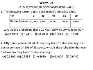
Warm-upCh.11 Inference for Linear Regression (Day 1) 1. The following is from a particular region’s mortality table. What is the probability that a 20-year-old will survive to be 60? (A) 0.1959 (B) 0.4419 (C) 0.7800 (D) 0.8041 (E) 0.9700 2. Fifty-three percent of adults say they have trouble sleeping. If a doctor contacts an SRS of 85 adults, what is the probability that over 55% will say they have trouble sleeping? (A) 0.3109 (B) 0.3558 (C) 0.3650 (D) 0.4000 (E) 0.6442
Answers to 3 and 4 of χ2 worksheet 3. The expected cell frequency for all 5 countries would be 616 for Necessary 234 for Unnecessary and 30 for Undecided. Step 1: The randomization condition is not met because the 1,000 person sample for each country is not specified to be random. It is questionable whether the 1,000 sampled are representative of each country.The count condition is met because there are counts for all cells of each category. The expected cell frequency is greater than 5 as shown above. The conditions are somewhat met for a Chi-Square model with 8 degrees of freedom for a test of homogeneity.
Step 2 and 3 Step 2: Ho: The proportion of opinions is distributed uniformly for all five countries. HA: The proportion of opinions is not uniformly distributed for all five counties. Step 3: χ2 = 1110.93 p-value ≈ 0 .
Step 4 and #4 Step 1 Step 4: The p-value is approximately zero. I reject the Ho. There is no similarity in the distribution of opinions of the five countries. The Chi square value of 1110.93 for 8 degrees of freedom demonstrates there is a drastic difference between expected observe. #4 Step 1: The sample of 5,387 is not random, but the sample is big enough to suspect of bias. The expected cell frequency is shown to be greater than five. There are counts for all cells of the categories. The conditions are met for a X2 model with 12 degrees of freedom with a test of independence.
Remaining steps are for #4 Step 2: Ho: Eye color is independent of hair color. HA: Eye color is not independent of hair color. Step 3: χ2 = 1241.06 p-value ≈ 0 . Step 4: I reject the Ho in favor of the HA. Eye color is not independent of hair color. With a p-value of approximately zero and a chi-square of 1241.06 there is strong evidence that these factors are not related.
Inference for Regression • Remember when we covered scatter plots was the least squares regression line. It included and the LSRL describes the set of numerical data in hopes of predicted the response variable for the given explanatory variable. • When sampling for different sets of data we know that there will be different that will affect the LSRL. • For inference of a regression line we will use called line of means or line of averages • Since there are two estimates, we will work with n – 2 degrees of freedom. • For the A.P. Statistics we are only interested in inference for slope (β).
Problem 1 (checking conditions only…for now) With the help of satellite images of Earth, craters from meteor impact, have been identified. Now more than 180 are known. These are only a small sample because many of the craters have been uncovered or eroded away. Astronomers have recognized roughly 35 million year cycle of cratering. Here’s a scatter plot of known impacts. Any ideas why both x and y axis are in log?
Checking Conditions • Linearity Assumption. The data on the scatter plot needs to demonstrate a linear relationship. • Randomization • *Equal Variance Condition. Looking at the residual plot the points need to be scattered constant throughout the line. No outliers or fan-shapes. • *Nearly Normal Condition. A histogram of the residuals and/or a normal plot needs to be evaluated. * There must be a residual plot and at least a residual plot to check the conditions.
Problem 2Checking conditions Enter data in L1 and L2, Then Stat, Calc select Lin Reg y = a +bx, LinReg L1, L2, Y1 Graph using Statplot function L1 and L2 and sketch the graph. For residual graph: Statplot, under YList go to List, Names and find Resid Graph and sketch plot. Then write if it meets all the conditions. To get the histogram of the residuals: Statplot, Select Histogram, X-List: Resid